Variational Auto-Encoder (VAE)

2024-06-09

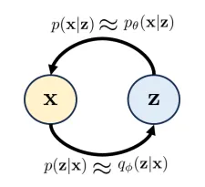
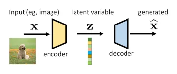
VAE can be considered as an encoder-decoder pair, the structure of which is shown as follows. VAE “Variational” comes from the fact that we use probability distribution to describe $\mathbf{x}$ and $\mathbf{z}$ . To see more details, we need to consider following distributions:

$p(\mathbf{x})$ : The distribution of $\mathbf{x}$ .
$p(\mathbf{z})$ : The distribution of latent variable. We make it a Gaussian $p(\mathbf{z})\sim \mathcal{N}(0, \mathbf{I})$ .
$p(\mathbf{z}|\mathbf{x})$ : The conditional distribution associated with the encoder.
$p(\mathbf{x}|\mathbf{z})$ : The conditional distribution associated with the decoder.

In practice, people often use the following two proxy distributions:

$q_{\phi}(\mathbf{z}|\mathbf{x})$ : The proxy for $p(\mathbf{z}|\mathbf{x})$ . We will make it Gaussian.
$p_{\theta}(\mathbf{x}|\mathbf{z})$ : The proxy for $p(\mathbf{x}|\mathbf{z})$ . We will also make it Gaussian. We don’t need to estimate anything for the Gaussian $p_{\theta}(\mathbf{x}|\mathbf{z})$ . Instead, we just use a decoder neural network to turn $\mathbf{z}$ back into $\mathbf{x}$ .

Evidence Lower Bound (ELBO)#

\text{ELBO}(\mathbf{x}) \overset{\text{def}}{=} \mathbb{E}_{q_{\phi}(\mathbf{z}|\mathbf{x})}\left[ \log \frac{p(\mathbf{x},\mathbf{z})}{q_{\phi}(\mathbf{z}|\mathbf{x})} \right]

ELBO is a lower bound for the prior distribution $\log p(\mathbf{x})$ . We can see that

\begin{align} \log p(x) &= \mathbb{E}_{q_{\phi}(\mathbf{z}|\mathbf{x})}[\log p(x)] \\ &=\mathbb{E}_{q_{\phi}(\mathbf{z}|\mathbf{x})}\left[ \log \frac{p(x,z)}{p(\mathbf{z}|\mathbf{x})} \right] \\ &=\mathbb{E}_{q_{\phi}(\mathbf{z}|\mathbf{x})}\left[ \log \frac{p(x,z)}{p(\mathbf{z}|\mathbf{x})} \times \frac{{q_{\phi}(\mathbf{z}|\mathbf{x})}}{q_{\phi}(\mathbf{z}|\mathbf{x})} \right] \\ &=\mathbb{E}_{q_{\phi}(\mathbf{z}|\mathbf{x})}\left[ \log \frac{p(\mathbf{x},\mathbf{z})}{q_{\phi}(\mathbf{z}|\mathbf{x})} \right] + \mathbb{E}_{q_{\phi}(\mathbf{z}|\mathbf{x})}\left[ \log \frac{q_{\phi}(\mathbf{z}|\mathbf{x})}{p(\mathbf{z}|\mathbf{x})} \right] \\ &=\text{ELBO}(x) + \mathbb{D}_{\text{KL}}(q_{\phi}(\mathbf{z}|\mathbf{x})||p(\mathbf{z}|\mathbf{x})) \\ &\geq \text{ELBO}(x) \end{align}

To make it more useful in practice, we use some tricks

\begin{align} \text{ELBO}(\mathbf{x}) &\overset{\text{def}}{=}\mathbb{E}_{q_{\phi}(\mathbf{z}|\mathbf{x})}\left[ \log \frac{p(\mathbf{x},\mathbf{z})}{q_{\phi}(\mathbf{z}|\mathbf{x})} \right] \\ &=\mathbb{E}_{q_{\phi}(\mathbf{z}|\mathbf{x})}\left[ \log \frac{{p(\mathbf{x|z}) p(\mathbf{z})}}{q_{\phi}(\mathbf{z|x})} \right] \\ &=\mathbb{E}_{q_{\phi}(\mathbf{z}|\mathbf{x})}[\log p(\mathbf{x|z})]+\mathbb{E}_{q_{\phi}(\mathbf{z}|\mathbf{x})}\left[ \log \frac{p(\mathbf{z})}{q_{\phi}(\mathbf{z|x})} \right] \\ &=\mathbb{E}_{q_{\phi}(\mathbf{z}|\mathbf{x})}[\log p_{\theta}(\mathbf{x|z})]-\mathbb{D}_{\text{KL}}(q_{\phi}(\mathbf{z}|\mathbf{x})||p(\mathbf{z})) \end{align}

Training VAE and Loss Function#

Let’s look at the decoder.

\hat{\mathbf{x}}=\text{decode}_{\theta}(\mathbf{z})

we make one more assumption that the error between the decoded image $\hat{\mathbf{x}}$ and the ground truth image $\mathbf{x}$ is Gaussian, which is $(\hat{\mathbf{x}}-\mathbf{x}) \sim \mathcal{N}(0, \sigma^{2}_{\text{dec}})$ for some $\sigma^{2}_{\text{dec}}$ . Then, it follows that the distribution $p_{\theta}(\mathbf{x}|\mathbf{z})$ is

\begin{aligned}\log p_{\boldsymbol{\theta}}(\mathbf{x}|\mathbf{z})&=\log\mathcal{N}(\mathbf{x}\mid\mathrm{decode}_{\boldsymbol{\theta}}(\mathbf{z}),\sigma_{\mathrm{dec}}^{2}\mathbf{I})\\&=\log\frac{1}{\sqrt{(2\pi\sigma_{\mathrm{dec}}^{2})^{D}}}\exp\left\{-\frac{\|\mathbf{x}-\mathrm{decode}_{\boldsymbol{\theta}}(\mathbf{z})\|^{2}}{2\sigma_{\mathrm{dec}}^{2}}\right\}\\&=-\frac{\|\mathbf{x}-\mathrm{decode}_{\boldsymbol{\theta}}(\mathbf{z})\|^{2}}{2\sigma_{\mathrm{dec}}^{2}}-\underbrace{\log\sqrt{(2\pi\sigma_{\mathrm{dec}}^{2})^{D}}}_{\text{you can ignore this term}}\end{aligned}

It is just the $\mathcal{l}_{2}$ loss between the decoded image and ground truth.

We approximate the expectation by Monte-Carlo simulation, then the loss function is

Training loss of VAE:

\operatorname*{argmax}_{\boldsymbol{\phi},\boldsymbol{\theta}}\left\{\frac{1}{L}\sum_{\ell=1}^{L}\log p_{\boldsymbol{\theta}}(\mathbf{x}^{(\ell)}|\mathbf{z}^{(\ell)})-\mathbb{D}_{\mathrm{KL}}(q_{\boldsymbol{\phi}}(\mathbf{z}|\mathbf{x}^{(\ell)})\|p(\mathbf{z}))\right\}

What’s more, the KL divergence for two $d$ -dimensional Gaussian distribution $\mathcal{N}(\boldsymbol{\mu}_{0},\boldsymbol{\Sigma}_{0})$ and $\mathcal{N}(\boldsymbol{\mu}_{1},\boldsymbol{\Sigma}_{1})$ is

\mathbb{D}_{\mathrm{KL}}(\mathcal{N}(\boldsymbol{\mu}_0,\boldsymbol{\Sigma}_0),\mathcal{N}(\boldsymbol{\mu}_1,\boldsymbol{\Sigma}_1))=\frac{1}{2}\left(\mathrm{Tr}(\boldsymbol{\Sigma}_1^{-1}\boldsymbol{\Sigma}_0)-d+(\boldsymbol{\mu}_1-\boldsymbol{\mu}_0)^T\boldsymbol{\Sigma}_1^{-1}(\boldsymbol{\mu}_1-\boldsymbol{\mu}_0)+\log\frac{\mathrm{det}\boldsymbol{\Sigma}_1}{\mathrm{det}\boldsymbol{\Sigma}_0}\right)

In our case, it can be simplified as follows:

\mathbb{D}_{\mathrm{KL}}(q_{\boldsymbol{\phi}}(\mathbf{z}|\mathbf{x}^{(\ell)})\parallel p(\mathbf{z}))=\frac{1}{2}\left((\sigma_{\boldsymbol{\phi}}^{2}(\mathbf{x}^{(\ell)}))^{d}+\boldsymbol{\mu}_{\boldsymbol{\phi}}(\mathbf{x}^{(\ell)})^{T}\boldsymbol{\mu}_{\boldsymbol{\phi}}(\mathbf{x}^{(\ell)})-d\log(\sigma_{\boldsymbol{\phi}}^{2}(\mathbf{x}^{(\ell)}))\right)

Reference#

[1] Chan, Stanley H. “Tutorial on Diffusion Models for Imaging and Vision.” arXiv preprint arXiv:2403.18103 (2024).