Explicit Score-Matching#

Suppose that we are given a dataset $\mathcal{X}=\{\mathbf{x}_1,\ldots,\mathbf{x}_M\}.$ The solution people came up with is to consider the classical kernel density estimation by defining a distribution

where $h$ is just some hyperparameter for the kernel function $K(\cdot)$, and $\mathbf{x}_m$ is the $m$-th sample in the training set.

• The sum of all these individual kernels gives us the overall kernel density estimate $q(\mathbf{x}).$
• The idea is similar to Gaussian Mixture Model.

Since $q(\mathbf{x})$ is an approximation to $p(\mathbf{x})$ which is never accessible, we can learn s$_{\boldsymbol{\theta}}(\mathbf{x})$ based on $q(\mathbf{x}).$ This leads to the following definition of the a loss function which can be used to train a network.

WARNING

The explicit score matching loss is

$$J_{\mathrm{ESM}}(\boldsymbol{\theta})\stackrel{\mathrm{def}}{=}\mathbb{E}_{q(\mathbf{x})}\|\mathrm{s}_{\boldsymbol{\theta}}(\mathbf{x})-\nabla_{\mathbf{x}}\log q(\mathbf{x})\|^2$$

By substituting the kernel density estimation, we can show that the loss is

Once we train the network s$_{\boldsymbol{\theta}}$, we can replace it in the Langevin dynamics equation to obtain the recursion:

Issue:

• The kernel density estimation is a fairly poor non-parameter estimation of the true distribution.
• When we have limited number of samples and the samples live in a high dimensional space, the kernel density estimation performance can be poor.

Denoising Score Matching#

In DSM, the loss function is defined as follows.

The idea comes from the Denoising Autoencoder approach of using pairs of clean and corrupted examples $(\mathbf{x},\mathbf{x}')$. In the generative model, $\mathbf{x}'$ can be seen as the $\mathbf{x}_{t}$.

The conditional distribution $q(\mathbf{x}|\mathbf{x}^{\prime})$ does not require an approximation. In the special case where $q(\mathbf{x}|\mathbf{x}^{\prime})=\mathcal{N}(\mathbf{x}\mid\mathbf{x}^{\prime},\sigma^2)$, we can let $\mathbf{x}=\mathbf{x}^\prime+\sigma\mathbf{z}.$ This will give us

As a result, the loss function of the denoising score matching becomes

The gradient operation cancels $\mathbf{x}$.

WARNING

The Denoising Score Matching has a loss function defined as

$$J_{\mathrm{DSM}}(\boldsymbol{\theta})=\mathbb{E}_{p(\mathbf{x})}\left[\frac12\left\|\mathbf{s}_{\boldsymbol{\theta}}(\mathbf{x}+\sigma\mathbf{z})+\frac{\mathbf{z}}{\sigma^2}\right\|^2\right]$$

• The quantity $\mathbf{x}+\sigma\mathbf{z}$ is effectively adding noise $\sigma\textbf{z}$ to a clean image $\mathbf{x}$.
• The score function $s_{{\boldsymbol{\theta}}}$ is supposed to take this noisy image and predict the noise $\frac {\mathbf{z} }{\sigma ^2}.$
• Predicting noise is equivalent to denoising, because any denoised image plus the predicted noise will give us the noisy observation.

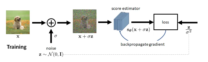
The training step can simply described as follows: You give us a training dataset $\{\mathbf{x}^{(\ell)}\}_{\ell=1}^L$, we train a network $\boldsymbol{\theta}$ with the goal to

The last thing is that why the loss function of DSM makes sense?

WARNING

Theorem For up to a constant $C$ which is independent of the variable $\boldsymbol{\theta}$, it holds that

$$J_{\mathrm{DSM}}(\theta)=J_{\mathrm{ESM}}(\theta)+C.$$

The proof is not hard.

For inference, we assume that we have already trained the score estimator s$_{\boldsymbol{\theta}}.$ To generate an image, we perform the following procedure for $t=1,\ldots,T{:}$