Diffusion models are incremental updates where the assembly of the whole gives us the encoder-decoder structure. The transition from one state to another is realized by a denoiser.
Structure variational diffusion model . The variational diffusion model has a sequence of states x 0 , x 1 , … , x T \mathbf{x}_{0},\mathbf{x}_{1},\dots,\mathbf{x}_{T} x 0 , x 1 , … , x T
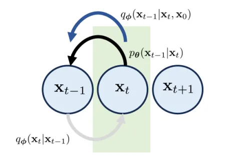
x 0 \mathbf{x}_{0} x 0 x T \mathbf{x}_{T} x T x T ∼ N ( 0 , I ) \mathbf{x}_{T}\sim \mathcal{N}(0, \mathbf{I}) x T ∼ N ( 0 , I ) x 1 , … , x T − 1 \mathbf{x}_{1},\dots,\mathbf{x}_{T-1} x 1 , … , x T − 1 1 Building Blocks# Transition Block# The t t t x t − 1 , x t \mathbf{x}_{t-1},\mathbf{x}_{t} x t − 1 , x t x t + 1 \mathbf{x_{t+1}} x t + 1
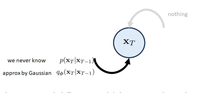
The forward transition ( x t − 1 → x t \mathbf{x}_{t-1}\to \mathbf{x}_{t} x t − 1 → x t p ( x t ∣ x t − 1 ) p(\mathbf{x}_{t}|\mathbf{x}_{t−1}) p ( x t ∣ x t − 1 ) Gaussian q ϕ ( x t ∣ x t − 1 ) q_{\phi}(\mathbf{x}_{t}|\mathbf{x}_{t-1}) q ϕ ( x t ∣ x t − 1 ) The reverse transition x t + 1 → x t \mathbf{x}_{t+1} \to \mathbf{x}_{t} x t + 1 → x t p ( x t + 1 ∣ x t ) p(\mathbf{x}_{t+1}|\mathbf{x}_{t}) p ( x t + 1 ∣ x t ) p θ ( x t + 1 ∣ x t ) p_{\theta}(\mathbf{x}_{t+1}|\mathbf{x}_{t}) p θ ( x t + 1 ∣ x t ) neural network ).
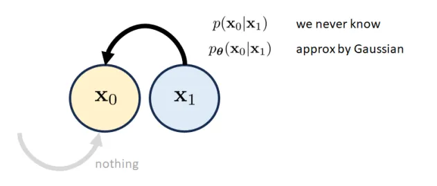
Initial Block: x 0 \mathbf{x}_{0} x 0 # We only need to worry about p ( x 0 ∣ x 1 ) p(\mathbf{x}_{0}|\mathbf{x}_{1}) p ( x 0 ∣ x 1 ) p θ ( x 0 ∣ x 1 ) p_{\theta}(\mathbf{x}_{0}|\mathbf{x}_{1}) p θ ( x 0 ∣ x 1 ) mean is computed through a neural network .
Final Block: x T \mathbf{x}_{T} x T # It should be a white Gaussian noise vector. The forward transition is approximated by q ϕ ( x T ∣ x T − 1 ) q_{\phi}(\mathbf{x}_{T} |\mathbf{x}_{T-1}) q ϕ ( x T ∣ x T − 1 ) Gaussian .
Understanding the Transition Distribution q ϕ ( x t ∣ x t − 1 ) q_{\phi}(\mathbf{x}_{t}|\mathbf{x}_{t-1}) q ϕ ( x t ∣ x t − 1 ) # In a DDPM model, the transition distribution q ϕ ( x t ∣ x t − 1 ) q_{\phi}(\mathbf{x}_{t}|\mathbf{x}_{t-1}) q ϕ ( x t ∣ x t − 1 )
q ϕ ( x t ∣ x t − 1 ) = d e f N ( x t ∣ α t x t − 1 , ( 1 − α t ) I ) q_{\boldsymbol{\phi}}(\mathbf{x}_t|\mathbf{x}_{t-1})\stackrel{\mathrm{def}}{=}\mathcal{N}(\mathbf{x}_t|\sqrt{\alpha_t}\mathbf{x}_{t-1},(1-\alpha_t)\mathbf{I}) q ϕ ( x t ∣ x t − 1 ) = def N ( x t ∣ α t x t − 1 , ( 1 − α t ) I ) The scaling factor α t \sqrt{ \alpha_{t} } α t It also means x t = α t x t − 1 + 1 − α t ϵ t − 1 \mathbf{x}_{t} = \sqrt{ \alpha_{t} }\mathbf{x}_{t-1}+\sqrt{ 1-\alpha_{t} }\epsilon_{t-1} x t = α t x t − 1 + 1 − α t ϵ t − 1 ϵ t − 1 ∼ N ( 0 , I ) \epsilon_{t-1}\sim \mathcal{N}(0,\mathbf{I}) ϵ t − 1 ∼ N ( 0 , I ) 2 The magical scalars α t \sqrt{ \alpha_{t} } α t 1 − α t 1-\alpha_{t} 1 − α t # Why α t \sqrt{ \alpha_{t} } α t 1 − α t 1-\alpha_{t} 1 − α t
q ϕ ( x t ∣ x t − 1 ) = N ( x t ∣ a x t − 1 , b 2 I ) . q_{\boldsymbol{\phi}}(\mathbf{x}_t|\mathbf{x}_{t-1})=\mathcal{N}(\mathbf{x}_t|a\mathbf{x}_{t-1},b^2\mathbf{I}). q ϕ ( x t ∣ x t − 1 ) = N ( x t ∣ a x t − 1 , b 2 I ) . where a ∈ R , b ∈ R a \in \mathbb{R}, b \in \mathbb{R} a ∈ R , b ∈ R
Proof. First, we have
x t = a x t − 1 + b ϵ t − 1 , w h e r e ϵ t − 1 ∼ N ( 0 , I ) . \mathbf{x}_t=a\mathbf{x}_{t-1}+b\boldsymbol{\epsilon}_{t-1},\quad\mathrm{where}\quad\boldsymbol{\epsilon}_{t-1}\sim\mathcal{N}(0,\mathbf{I}). x t = a x t − 1 + b ϵ t − 1 , where ϵ t − 1 ∼ N ( 0 , I ) . Then, we carry on the recursion
x t = a x t − 1 + b ϵ t − 1 = a ( a x t − 2 + b ϵ t − 2 ) + b ϵ t − 1 = a 2 x t − 2 + a b ϵ t − 2 + b ϵ t − 1 = : = a t x 0 + b [ ϵ t − 1 + a ϵ t − 2 + a 2 ϵ t − 3 + … + a t − 1 ϵ 0 ] ⏟ = d e f w t . \begin{aligned} \mathbf{x}_{t}& =a\mathbf{x}_{t-1}+b\boldsymbol{\epsilon}_{t-1} \\ &=a(a\mathbf{x}_{t-2}+b\boldsymbol{\epsilon}_{t-2})+b\boldsymbol{\epsilon}_{t-1} \\ &=a^2\mathbf{x}_{t-2}+ab\boldsymbol{\epsilon}_{t-2}+b\boldsymbol{\epsilon}_{t-1} \\ &=: \\ &=a^t\mathbf{x}_0+b\underbrace{\left[\boldsymbol{\epsilon}_{t-1}+a\boldsymbol{\epsilon}_{t-2}+a^2\boldsymbol{\epsilon}_{t-3}+\ldots+a^{t-1}\boldsymbol{\epsilon}_0\right]}_{\overset{\mathrm{def}}{\operatorname*{=}}\mathbf{w}_t}. \end{aligned} x t = a x t − 1 + b ϵ t − 1 = a ( a x t − 2 + b ϵ t − 2 ) + b ϵ t − 1 = a 2 x t − 2 + ab ϵ t − 2 + b ϵ t − 1 =: = a t x 0 + b = def w t [ ϵ t − 1 + a ϵ t − 2 + a 2 ϵ t − 3 + … + a t − 1 ϵ 0 ] . It is clear that E [ w t ] = 0 \mathbb{E}[\mathbf{w}_{t}]=0 E [ w t ] = 0
C o v [ w t ] = d e f b 2 ( C o v ( ϵ t − 1 ) + a 2 C o v ( ϵ t − 2 ) + … + ( a t − 1 ) 2 C o v ( ϵ 0 ) ) = b 2 ( 1 + a 2 + a 4 + … + a 2 ( t − 1 ) ) I = b 2 ⋅ 1 − a 2 t 1 − a 2 I . \begin{aligned} \mathrm{Cov}[\mathbf{w}_{t}]&\stackrel{\mathrm{def}}{=} b^{2}(\mathrm{Cov}(\boldsymbol{\epsilon}_{t-1})+a^{2}\mathrm{Cov}(\boldsymbol{\epsilon}_{t-2})+\ldots+(a^{t-1})^{2}\mathrm{Cov}(\boldsymbol{\epsilon}_{0})) \\ &=b^2(1+a^2+a^4+\ldots+a^{2(t-1)})\mathbf{I} \\ &=b^2\cdot\frac{1-a^{2t}}{1-a^2}\mathbf{I}. \end{aligned} Cov [ w t ] = def b 2 ( Cov ( ϵ t − 1 ) + a 2 Cov ( ϵ t − 2 ) + … + ( a t − 1 ) 2 Cov ( ϵ 0 )) = b 2 ( 1 + a 2 + a 4 + … + a 2 ( t − 1 ) ) I = b 2 ⋅ 1 − a 2 1 − a 2 t I . As t → ∞ , a t → 0 t\to\infty,a^t\to0 t → ∞ , a t → 0 0 < a < 1. 0<a<1. 0 < a < 1. t = ∞ t=\infty t = ∞ lim t → ∞ C o v [ w t ] = b 2 1 − a 2 I . \lim\limits_{t\to\infty}\mathrm{Cov}[\mathbf{w}_t]=\frac{b^2}{1-a^2}\mathbf{I}. t → ∞ lim Cov [ w t ] = 1 − a 2 b 2 I . lim t → ∞ Cov [ w t ] = I \lim_{t\to\infty}\text{Cov}[\mathbf{w}_t]=\mathbf{I} lim t → ∞ Cov [ w t ] = I x t \mathbf{x}_t x t N ( 0 , I ) \mathcal{N}(0,\mathbf{I}) N ( 0 , I ) b = 1 − a 2 b=\sqrt{1-a^{2}} b = 1 − a 2
Now, if we let a = α a=\sqrt{\alpha} a = α b = 1 − α . b=\sqrt1-\alpha. b = 1 − α .
x t = α x t − 1 + 1 − α ϵ t − 1 \mathbf{x}_t=\sqrt{\alpha}\mathbf{x}_{t-1}+\sqrt{1-\alpha}\boldsymbol{\epsilon}_{t-1} x t = α x t − 1 + 1 − α ϵ t − 1 Or equivalently, q ϕ ( x ∣ x t − 1 ) = N ( x t ∣ α x t − 1 , ( 1 − α ) I ) . q_{\boldsymbol{\phi}}(\mathbf{x}|\mathbf{x}_{t-1})=\mathcal{N}(\mathbf{x}_{t}\mid\sqrt{\alpha}\mathbf{x}_{t-1},(1-\alpha)\mathbf{I}). q ϕ ( x ∣ x t − 1 ) = N ( x t ∣ α x t − 1 , ( 1 − α ) I ) . α \alpha α α t \alpha_t α t
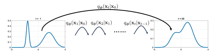
3 Distribution q ϕ ( x t ∣ x 0 ) q_{\phi}(\mathbf{x}_{t}|\mathbf{x}_{0}) q ϕ ( x t ∣ x 0 ) # Conditional distribution q ϕ ( x t ∣ x 0 ) q_{\phi}(\mathbf{x}_{t}|\mathbf{x}_{0}) q ϕ ( x t ∣ x 0 )
q ϕ ( x t ∣ x 0 ) = N ( x t ∣ α ‾ t x 0 , ( 1 − α ‾ t ) I ) , q_{\boldsymbol{\phi}}(\mathbf{x}_{t}|\mathbf{x}_{0})=\mathcal{N}(\mathbf{x}_{t}\mid\sqrt{\overline{\alpha}_{t}}\mathbf{x}_{0},(1-\overline{\alpha}_{t})\mathbf{I}), q ϕ ( x t ∣ x 0 ) = N ( x t ∣ α t x 0 , ( 1 − α t ) I ) , where α ‾ t = ∏ i = 1 t α i \overline{\alpha}_{t}=\prod_{i=1}^{t}\alpha_{i} α t = ∏ i = 1 t α i
Proof.
x t = α t x t − 1 + 1 − α t ϵ t − 1 = α t ( α t − 1 x t − 2 + 1 − α t − 1 ϵ t − 2 ) + 1 − α t ϵ t − 1 = α t α t − 1 x t − 2 + α t 1 − α t − 1 ϵ t − 2 + 1 − α t ϵ t − 1 ⏟ w 1 . \begin{aligned}\mathbf{x}_{t}&=\sqrt{\alpha_t}\mathbf{x}_{t-1}+\sqrt{1-\alpha_t}\boldsymbol{\epsilon}_{t-1}\\&=\sqrt{\alpha_t}(\sqrt{\alpha_{t-1}}\mathbf{x}_{t-2}+\sqrt{1-\alpha_{t-1}}\boldsymbol{\epsilon}_{t-2})+\sqrt{1-\alpha_t}\boldsymbol{\epsilon}_{t-1}\\&=\sqrt{\alpha_t\alpha_{t-1}}\mathbf{x}_{t-2}+\underbrace{\sqrt{\alpha_t}\sqrt{1-\alpha_{t-1}}\boldsymbol{\epsilon}_{t-2}+\sqrt{1-\alpha_t}\boldsymbol{\epsilon}_{t-1}}_{\mathbf{w}_1}.\end{aligned} x t = α t x t − 1 + 1 − α t ϵ t − 1 = α t ( α t − 1 x t − 2 + 1 − α t − 1 ϵ t − 2 ) + 1 − α t ϵ t − 1 = α t α t − 1 x t − 2 + w 1 α t 1 − α t − 1 ϵ t − 2 + 1 − α t ϵ t − 1 . The new covariance is
E [ w 1 w 1 T ] = [ ( α t 1 − α t − 1 ) 2 + ( 1 − α t ) 2 ] I = [ α t ( 1 − α t − 1 ) + 1 − α t ] I = [ 1 − α t α t − 1 ] I . \begin{aligned}\mathbb{E}[\mathbf{w}_{1}\mathbf{w}_{1}^{T}]&=[(\sqrt{\alpha_{t}}\sqrt{1-\alpha_{t-1}})^{2}+(\sqrt{1-\alpha_{t}})^{2}]\mathbf{I}\\&=[\alpha_t(1-\alpha_{t-1})+1-\alpha_t]\mathbf{I}=[1-\alpha_t\alpha_{t-1}]\mathbf{I}.\end{aligned} E [ w 1 w 1 T ] = [( α t 1 − α t − 1 ) 2 + ( 1 − α t ) 2 ] I = [ α t ( 1 − α t − 1 ) + 1 − α t ] I = [ 1 − α t α t − 1 ] I . We can show that the recursion is updated to become a linear combination of x t − 2 \mathbf{x}_{t-2} x t − 2 ϵ t − 2 : \boldsymbol\epsilon_t-2: ϵ t − 2 :
x t = α t α t − 1 x t − 2 + 1 − α t α t − 1 ϵ t − 2 = α t α t − 1 α t − 2 x t − 3 + 1 − α t α t − 1 α t − 2 ϵ t − 3 = ⋮ = ∏ i = 1 t α i x 0 + 1 − ∏ i = 1 t α i ϵ 0 . \begin{aligned}\mathbf{x}_{t}&=\sqrt{\alpha_{t}\alpha_{t-1}}\mathbf{x}_{t-2}+\sqrt{1-\alpha_{t}\alpha_{t-1}}\boldsymbol{\epsilon}_{t-2}\\&=\sqrt{\alpha_{t}\alpha_{t-1}\alpha_{t-2}}\mathbf{x}_{t-3}+\sqrt{1-\alpha_{t}\alpha_{t-1}\alpha_{t-2}}\boldsymbol{\epsilon}_{t-3}\\&=\vdots\\&=\sqrt{\prod_{i=1}^t\alpha_i}\mathbf{x}_0+\sqrt{1-\prod_{i=1}^t\alpha_i}\boldsymbol{\epsilon}_0.\end{aligned} x t = α t α t − 1 x t − 2 + 1 − α t α t − 1 ϵ t − 2 = α t α t − 1 α t − 2 x t − 3 + 1 − α t α t − 1 α t − 2 ϵ t − 3 = ⋮ = i = 1 ∏ t α i x 0 + 1 − i = 1 ∏ t α i ϵ 0 . So, if we define α ‾ t = ∏ i = 1 t α i \overline{\alpha}_t=\prod_{i=1}^t\alpha_i α t = ∏ i = 1 t α i
x t = α ‾ t x 0 + 1 − α ‾ t ϵ 0 . \mathbf{x}_{t}=\sqrt{\overline{\alpha}_{t}}\mathbf{x}_{0}+\sqrt{1-\overline{\alpha}_{t}}\epsilon_{0}. x t = α t x 0 + 1 − α t ϵ 0 . In other words, the distribution q ϕ ( x t ∣ x 0 ) q_{\boldsymbol{\phi}}(\mathbf{x}_{t}|\mathbf{x}_{0}) q ϕ ( x t ∣ x 0 )
x t ∼ q ϕ ( x t ∣ x 0 ) = N ( x t ∣ α ‾ t x 0 , ( 1 − α ‾ t ) I ) . \mathbf{x}_t\sim q_{\boldsymbol{\phi}}(\mathbf{x}_t|\mathbf{x}_0)=\mathcal{N}(\mathbf{x}_t\:|\:\sqrt{\overline{\alpha}_t}\mathbf{x}_0,\:(1-\overline{\alpha}_t)\mathbf{I}). x t ∼ q ϕ ( x t ∣ x 0 ) = N ( x t ∣ α t x 0 , ( 1 − α t ) I ) .
4 Evidence Lower Bound# The ELBO for the variational diffusion model is
E L B O ϕ , θ ( x ) = E q ϕ ( x 1 ∣ x 0 ) [ log p θ ( x 0 ∣ x 1 ) ⏟ h o w g o o d t h e i n i t i a l b l o c k i s ] − E q ϕ ( x T − 1 ∣ x 0 ) [ D K L ( q ϕ ( x T ∣ x T − 1 ) ∥ p ( x T ) ) ⏟ how good the final block is ] − ∑ t = 1 T − 1 E q ϕ ( x t − 1 , x t + 1 ∣ x 0 ) [ D K L ( q ϕ ( x t ∣ x t − 1 ) ∥ p θ ( x t ∣ x t + 1 ) ) ⏟ h o w g o o d t h e t r a n s i t i o n b l o c k s a r e ] \begin{aligned} \mathrm{ELBO}_{\phi,\theta}(\mathbf{x})= &\mathbb{E}_{q_{\boldsymbol{\phi}}(\mathbf{x}_{1}|\mathbf{x}_{0})}\bigg[\log\underbrace{p_{\boldsymbol{\theta}}(\mathbf{x}_{0}|\mathbf{x}_{1})}_{\mathrm{how~good~the~initial~block~is}}\bigg] \\ &-\mathbb{E}_{q_{\boldsymbol{\phi}}(\mathbf{x}_{T-1}|\mathbf{x}_{0})}\left[\underbrace{\mathbb{D}_{\mathrm{KL}}\left(q_{\boldsymbol{\phi}}(\mathbf{x}_{T}|\mathbf{x}_{T-1})\|p(\mathbf{x}_{T})\right)}_{\text{how good the final block is}}\right] \\ &-\sum_{t=1}^{T-1}\mathbb{E}_{q_{\boldsymbol{\phi}}(\mathbf{x}_{t-1},\mathbf{x}_{t+1}|\mathbf{x}_{0})}\Big[\underbrace{\mathbb{D}_{\mathrm{KL}}\Big(q_{\boldsymbol{\phi}}(\mathbf{x}_{t}|\mathbf{x}_{t-1})\|p_{\boldsymbol{\theta}}(\mathbf{x}_{t}|\mathbf{x}_{t+1})\Big)}_{\mathrm{how~good~the~transition~blocks~are}}\Big] \end{aligned} ELBO ϕ , θ ( x ) = E q ϕ ( x 1 ∣ x 0 ) [ log how good the initial block is p θ ( x 0 ∣ x 1 ) ] − E q ϕ ( x T − 1 ∣ x 0 ) how good the final block is D KL ( q ϕ ( x T ∣ x T − 1 ) ∥ p ( x T ) ) − t = 1 ∑ T − 1 E q ϕ ( x t − 1 , x t + 1 ∣ x 0 ) [ how good the transition blocks are D KL ( q ϕ ( x t ∣ x t − 1 ) ∥ p θ ( x t ∣ x t + 1 ) ) ] Interpretation of ELBO:
Reconstruction. Use log-likelihood p θ ( x 0 ∣ x 1 ) p_{\theta}(\mathbf{x}_{0}|\mathbf{x}_{1}) p θ ( x 0 ∣ x 1 ) Prior Matching. Use KL divergence to measure the difference between q ϕ ( x T ∣ x T − 1 ) q_{\phi}(\mathbf{x}_{T}|\mathbf{x}_{T −1}) q ϕ ( x T ∣ x T − 1 ) p ( x T ) p(\mathbf{x}_{T}) p ( x T ) Consistency. The forward transition is determined by the distribution q ϕ ( x t ∣ x t − 1 ) q_{\phi}(\mathbf{x}_{t}|\mathbf{x}_{t-1}) q ϕ ( x t ∣ x t − 1 ) reverse transition is determined by the neural network p θ ( x t ∣ x t + 1 ) . p_{\boldsymbol{\theta}}(\mathbf{x}_{t}|\mathbf{x}_{t+1}). p θ ( x t ∣ x t + 1 ) . KL divergence to measure the deviation.Proof.
log p ( x ) = log p ( x 0 ) = log ∫ p ( x 0 : T ) d x 1 : T = log ∫ p ( x 0 : T ) q ϕ ( x 1 : T ∣ x 0 ) q ϕ ( x 1 : T ∣ x 0 ) d x 1 : T = log ∫ q ϕ ( x 1 : T ∣ x 0 ) [ p ( x 0 : T ) q ϕ ( x 1 : T ∣ x 0 ) ] d x 1 : T = log E q ϕ ( x 1 : T ∣ x 0 ) [ p ( x 0 : T ) q ϕ ( x 1 : T ∣ x 0 ) ] ≥ E q ϕ ( x 1 : T ∣ x 0 ) [ log p ( x 0 : T ) q ϕ ( x 1 : T ∣ x 0 ) ] \begin{aligned} \operatorname{log}p(\mathbf{x})& =\log p(\mathbf{x}_{0}) \\ &=\log\int p(\mathbf{x}_{0:T})d\mathbf{x}_{1:T} \\ &=\log\int p(\mathbf{x}_{0:T})\frac{q_{\boldsymbol{\phi}}(\mathbf{x}_{1:T}|\mathbf{x}_{0})}{q_{\boldsymbol{\phi}}(\mathbf{x}_{1:T}|\mathbf{x}_{0})}d\mathbf{x}_{1:T} \\ &=\log\int q_{\boldsymbol{\phi}}(\mathbf{x}_{1:T}|\mathbf{x}_{0})\left[\frac{p(\mathbf{x}_{0:T})}{q_{\boldsymbol{\phi}}(\mathbf{x}_{1:T}|\mathbf{x}_{0})}\right]d\mathbf{x}_{1:T} \\ &=\log\mathbb{E}_{q_{\boldsymbol{\phi}}(\mathbf{x}_{1:T}|\mathbf{x}_{0})}\left[\frac{p(\mathbf{x}_{0:T})}{q_{\boldsymbol{\phi}}(\mathbf{x}_{1:T}|\mathbf{x}_{0})}\right]\\ &\geq \mathbb{E}_{q_{\boldsymbol{\phi}}(\mathbf{x}_{1:T}|\mathbf{x}_{0})}\left[\log\frac{p(\mathbf{x}_{0:T})}{q_{\boldsymbol{\phi}}(\mathbf{x}_{1:T}|\mathbf{x}_{0})}\right] \end{aligned} log p ( x ) = log p ( x 0 ) = log ∫ p ( x 0 : T ) d x 1 : T = log ∫ p ( x 0 : T ) q ϕ ( x 1 : T ∣ x 0 ) q ϕ ( x 1 : T ∣ x 0 ) d x 1 : T = log ∫ q ϕ ( x 1 : T ∣ x 0 ) [ q ϕ ( x 1 : T ∣ x 0 ) p ( x 0 : T ) ] d x 1 : T = log E q ϕ ( x 1 : T ∣ x 0 ) [ q ϕ ( x 1 : T ∣ x 0 ) p ( x 0 : T ) ] ≥ E q ϕ ( x 1 : T ∣ x 0 ) [ log q ϕ ( x 1 : T ∣ x 0 ) p ( x 0 : T ) ] The last inequality follows from Jensen’s inequality. Note that
p ( x 0 : T ) = p ( x T ) ∏ t = 1 T p ( x t − 1 ∣ x t ) = p ( x T ) p ( x 0 ∣ x 1 ) ∏ t = 2 T p ( x t − 1 ∣ x t ) p(\mathbf{x}_{0:T})=p(\mathbf{x}_T)\prod_{t=1}^Tp(\mathbf{x}_{t-1}|\mathbf{x}_t)=p(\mathbf{x}_T)p(\mathbf{x}_0|\mathbf{x}_1)\prod_{t=2}^Tp(\mathbf{x}_{t-1}|\mathbf{x}_t) p ( x 0 : T ) = p ( x T ) t = 1 ∏ T p ( x t − 1 ∣ x t ) = p ( x T ) p ( x 0 ∣ x 1 ) t = 2 ∏ T p ( x t − 1 ∣ x t ) q ϕ ( x 1 : T ∣ x 0 ) = ∏ t = 1 T q ϕ ( x t ∣ x t − 1 ) = q ϕ ( x T ∣ x T − 1 ) ∏ t = 1 T − 1 q ϕ ( x t ∣ x t − 1 ) . q_{\boldsymbol{\phi}}(\mathbf{x}_{1:T}|\mathbf{x}_0)=\prod_{t=1}^Tq_{\boldsymbol{\phi}}(\mathbf{x}_t|\mathbf{x}_{t-1})=q_{\boldsymbol{\phi}}(\mathbf{x}_T|\mathbf{x}_{T-1})\prod_{t=1}^{T-1}q_{\boldsymbol{\phi}}(\mathbf{x}_t|\mathbf{x}_{t-1}). q ϕ ( x 1 : T ∣ x 0 ) = t = 1 ∏ T q ϕ ( x t ∣ x t − 1 ) = q ϕ ( x T ∣ x T − 1 ) t = 1 ∏ T − 1 q ϕ ( x t ∣ x t − 1 ) . Then
log p ( x ) ≥ E q ϕ ( x 1 : T ∣ x 0 ) [ log p ( x 0 : T ) q ϕ ( x 1 : T ∣ x 0 ) ] = E q ϕ ( x 1 : T ∣ x 0 ) [ log p ( x T ) p ( x 0 ∣ x 1 ) ∏ t = 2 T p ( x t − 1 ∣ x t ) q ϕ ( x T ∣ x T − 1 ) ∏ t = 1 T − 1 q ϕ ( x t ∣ x t − 1 ) ] = E q ϕ ( x 1 : T ∣ x 0 ) [ log p ( x T ) p ( x 0 ∣ x 1 ) ∏ t = 1 T − 1 p ( x t ∣ x t + 1 ) q ϕ ( x T ∣ x T − 1 ) ∏ t = 1 T − 1 q ϕ ( x t ∣ x t − 1 ) ] = E q ϕ ( x 1 : T ∣ x 0 ) [ log p ( x T ) p ( x 0 ∣ x 1 ) q ϕ ( x T ∣ x T − 1 ) ] + E q ϕ ( x 1 : T ∣ x 0 ) [ log ∏ t = 1 T − 1 p ( x t ∣ x t + 1 ) q ϕ ( x t ∣ x t − 1 ) ] \begin{aligned} \operatorname{log}p(\mathbf{x})& \geq\mathbb{E}_{q_{\boldsymbol{\phi}}(\mathbf{x}_{1:T}|\mathbf{x}_{0})}\left[\log\frac{p(\mathbf{x}_{0:T})}{q_{\boldsymbol{\phi}}(\mathbf{x}_{1:T}|\mathbf{x}_{0})}\right] \\ &=\mathbb{E}_{q_{\boldsymbol{\phi}}(\mathbf{x}_{1:T}|\mathbf{x}_0)}\left[\log\frac{p(\mathbf{x}_T)p(\mathbf{x}_0|\mathbf{x}_1)\prod_{t=2}^Tp(\mathbf{x}_{t-1}|\mathbf{x}_t)}{q_{\boldsymbol{\phi}}(\mathbf{x}_T|\mathbf{x}_{T-1})\prod_{t=1}^{T-1}q_{\boldsymbol{\phi}}(\mathbf{x}_t|\mathbf{x}_{t-1})}\right] \\ &=\mathbb{E}_{q_{\boldsymbol{\phi}}(\mathbf{x}_{1:T}|\mathbf{x}_0)}\left[\log\frac{p(\mathbf{x}_T)p(\mathbf{x}_0|\mathbf{x}_1)\prod_{t=1}^{T-1}p(\mathbf{x}_t|\mathbf{x}_{t+1})}{q_{\boldsymbol{\phi}}(\mathbf{x}_T|\mathbf{x}_{T-1})\prod_{t=1}^{T-1}q_{\boldsymbol{\phi}}(\mathbf{x}_t|\mathbf{x}_{t-1})}\right] \\ &=\mathbb{E}_{q_{\boldsymbol{\phi}}(\mathbf{x}_{1:T}|\mathbf{x}_{0})}\left[\log\frac{p(\mathbf{x}_{T})p(\mathbf{x}_{0}|\mathbf{x}_{1})}{q_{\boldsymbol{\phi}}(\mathbf{x}_{T}|\mathbf{x}_{T-1})}\right]+\mathbb{E}_{q_{\boldsymbol{\phi}}(\mathbf{x}_{1:T}|\mathbf{x}_{0})}\left[\log\prod_{t=1}^{T-1}\frac{p(\mathbf{x}_{t}|\mathbf{x}_{t+1})}{q_{\boldsymbol{\phi}}(\mathbf{x}_{t}|\mathbf{x}_{t-1})}\right] \end{aligned} log p ( x ) ≥ E q ϕ ( x 1 : T ∣ x 0 ) [ log q ϕ ( x 1 : T ∣ x 0 ) p ( x 0 : T ) ] = E q ϕ ( x 1 : T ∣ x 0 ) [ log q ϕ ( x T ∣ x T − 1 ) ∏ t = 1 T − 1 q ϕ ( x t ∣ x t − 1 ) p ( x T ) p ( x 0 ∣ x 1 ) ∏ t = 2 T p ( x t − 1 ∣ x t ) ] = E q ϕ ( x 1 : T ∣ x 0 ) [ log q ϕ ( x T ∣ x T − 1 ) ∏ t = 1 T − 1 q ϕ ( x t ∣ x t − 1 ) p ( x T ) p ( x 0 ∣ x 1 ) ∏ t = 1 T − 1 p ( x t ∣ x t + 1 ) ] = E q ϕ ( x 1 : T ∣ x 0 ) [ log q ϕ ( x T ∣ x T − 1 ) p ( x T ) p ( x 0 ∣ x 1 ) ] + E q ϕ ( x 1 : T ∣ x 0 ) [ log t = 1 ∏ T − 1 q ϕ ( x t ∣ x t − 1 ) p ( x t ∣ x t + 1 ) ] The Reconstruction term can be simplified as
E q ϕ ( x 1 : T ∣ x 0 ) [ log p ( x 0 ∣ x 1 ) ] = E q ϕ ( x 1 ∣ x 0 ) [ log p ( x 0 ∣ x 1 ) ] , \mathbb{E}_{q_{\boldsymbol{\phi}}(\mathbf{x}_{1:T}|\mathbf{x}_0)}\bigg[\log p(\mathbf{x}_0|\mathbf{x}_1)\bigg]=\mathbb{E}_{q_{\boldsymbol{\phi}}(\mathbf{x}_1|\mathbf{x}_0)}\bigg[\log p(\mathbf{x}_0|\mathbf{x}_1)\bigg], E q ϕ ( x 1 : T ∣ x 0 ) [ log p ( x 0 ∣ x 1 ) ] = E q ϕ ( x 1 ∣ x 0 ) [ log p ( x 0 ∣ x 1 ) ] , where we used the fact that the conditioning x 1 : T ∣ x 0 \mathbf{x}_1:T|\mathbf{x}_0 x 1 : T ∣ x 0 x 1 ∣ x 0 . \mathbf{x}_1|\mathbf{x}_0. x 1 ∣ x 0 .
E q ϕ ( x 1 : T ∣ x 0 ) [ log p ( x T ) q ϕ ( x T ∣ x T − 1 ) ] = E q ϕ ( x T , x T − 1 ∣ x 0 ) [ log p ( x T ) q ϕ ( x T ∣ x T − 1 ) ] = − E q ϕ ( x T − 1 , x T ∣ x 0 ) [ D K L ( q ϕ ( x T ∣ x T − 1 ) ∥ p ( x T ) ) ] , \begin{aligned}\mathbb{E}_{q_{\boldsymbol{\phi}}(\mathbf{x}_{1:T}|\mathbf{x}_{0})}\left[\log\frac{p(\mathbf{x}_{T})}{q_{\boldsymbol{\phi}}(\mathbf{x}_{T}|\mathbf{x}_{T-1})}\right]&=\mathbb{E}_{q_{\boldsymbol{\phi}}(\mathbf{x}_{T},\mathbf{x}_{T-1}|\mathbf{x}_{0})}\left[\log\frac{p(\mathbf{x}_{T})}{q_{\boldsymbol{\phi}}(\mathbf{x}_{T}|\mathbf{x}_{T-1})}\right]\\&=-\mathbb{E}_{q_{\boldsymbol{\phi}}(\mathbf{x}_{T-1},\mathbf{x}_{T}|\mathbf{x}_{0})}\bigg[\mathbb{D}_{\mathrm{KL}}\left(q_{\boldsymbol{\phi}}(\mathbf{x}_{T}|\mathbf{x}_{T-1})\|p(\mathbf{x}_{T})\right)\bigg],\end{aligned} E q ϕ ( x 1 : T ∣ x 0 ) [ log q ϕ ( x T ∣ x T − 1 ) p ( x T ) ] = E q ϕ ( x T , x T − 1 ∣ x 0 ) [ log q ϕ ( x T ∣ x T − 1 ) p ( x T ) ] = − E q ϕ ( x T − 1 , x T ∣ x 0 ) [ D KL ( q ϕ ( x T ∣ x T − 1 ) ∥ p ( x T ) ) ] , Finally, we can show that
E q ϕ ( x 1 : T ∣ x 0 ) [ log ∏ t = 1 T − 1 p ( x t ∣ x t + 1 ) q ϕ ( x t ∣ x t − 1 ) ] = ∑ t = 1 T − 1 E q ϕ ( x 1 : T ∣ x 0 ) [ log p ( x t ∣ x t + 1 ) q ϕ ( x t ∣ x t − 1 ) ] = ∑ t = 1 T − 1 E q ϕ ( x t − 1 , x t , x t + 1 ∣ x 0 ) [ log p ( x t ∣ x t + 1 ) q ϕ ( x t ∣ x t − 1 ) ] = − ∑ t = 1 T − 1 E q ϕ ( x t − 1 , x t + 1 ∣ x 0 ) [ D K L ( q ϕ ( x t ∣ x t − 1 ) ∥ p ( x t ∣ x t + 1 ) ) ] ⏟ consistency . \begin{aligned} \mathbb{E}_{q_{\boldsymbol{\phi}}(\mathbf{x}_{1:T}|\mathbf{x}_0)}\left[\log\prod_{t=1}^{T-1}\frac{p(\mathbf{x}_t|\mathbf{x}_{t+1})}{q_{\boldsymbol{\phi}}(\mathbf{x}_t|\mathbf{x}_{t-1})}\right] &=\sum_{t=1}^{T-1}\mathbb{E}_{q_{\boldsymbol{\phi}}(\mathbf{x}_{1:T}|\mathbf{x}_{0})}\left[\log\frac{p(\mathbf{x}_{t}|\mathbf{x}_{t+1})}{q_{\boldsymbol{\phi}}(\mathbf{x}_{t}|\mathbf{x}_{t-1})}\right] \\ &=\sum_{t=1}^{T-1}\mathbb{E}_{q_{\boldsymbol{\phi}}(\mathbf{x}_{t-1},\mathbf{x}_{t},\mathbf{x}_{t+1}|\mathbf{x}_{0})}\left[\log\frac{p(\mathbf{x}_{t}|\mathbf{x}_{t+1})}{q_{\boldsymbol{\phi}}(\mathbf{x}_{t}|\mathbf{x}_{t-1})}\right] \\ &=\underbrace{-\sum_{t=1}^{T-1}\mathbb{E}_{q_{\boldsymbol{\phi}}(\mathbf{x}_{t-1},\mathbf{x}_{t+1}|\mathbf{x}_{0})}\left[\mathbb{D}_{\mathrm{KL}}\left(q_{\boldsymbol{\phi}}(\mathbf{x}_{t}|\mathbf{x}_{t-1})\|p(\mathbf{x}_{t}|\mathbf{x}_{t+1})\right)\right]}_{\text{consistency}}. \end{aligned} E q ϕ ( x 1 : T ∣ x 0 ) [ log t = 1 ∏ T − 1 q ϕ ( x t ∣ x t − 1 ) p ( x t ∣ x t + 1 ) ] = t = 1 ∑ T − 1 E q ϕ ( x 1 : T ∣ x 0 ) [ log q ϕ ( x t ∣ x t − 1 ) p ( x t ∣ x t + 1 ) ] = t = 1 ∑ T − 1 E q ϕ ( x t − 1 , x t , x t + 1 ∣ x 0 ) [ log q ϕ ( x t ∣ x t − 1 ) p ( x t ∣ x t + 1 ) ] = consistency − t = 1 ∑ T − 1 E q ϕ ( x t − 1 , x t + 1 ∣ x 0 ) [ D KL ( q ϕ ( x t ∣ x t − 1 ) ∥ p ( x t ∣ x t + 1 ) ) ] . By replacing p ( x 0 ∣ x 1 ) p(\mathbf{x}_0|\mathbf{x}_1) p ( x 0 ∣ x 1 ) p θ ( x 0 ∣ x 1 ) p_{\boldsymbol{\theta}}(\mathbf{x}_0|\mathbf{x}_1) p θ ( x 0 ∣ x 1 ) p ( x t ∣ x t + 1 ) p(\mathbf{x}_t|\mathbf{x}_{t+1}) p ( x t ∣ x t + 1 ) p θ ( x t ∣ x t + 1 ) p_{\boldsymbol{\theta}}(\mathbf{x}_t|\mathbf{x}_{t+1}) p θ ( x t ∣ x t + 1 )
5 Rewrite the Consistency Term# The difficulty above is that we need to draw samples ( x t − 1 , x t + 1 ) (\mathbf{x}_{t-1},\mathbf{x}_{t+1}) ( x t − 1 , x t + 1 ) q ϕ ( x t − 1 , x t + 1 ∣ x 0 ) q_{\phi}(\mathbf{x}_{t-1},\mathbf{x}_{t+1}|\mathbf{x}_{0}) q ϕ ( x t − 1 , x t + 1 ∣ x 0 )
With Bayes theorem:
q ( x t ∣ x t − 1 ) = q ( x t − 1 ∣ x t ) q ( x t ) q ( x t − 1 ) ⟹ condition on x 0 q ( x t ∣ x t − 1 , x 0 ) = q ( x t − 1 ∣ x t , x 0 ) q ( x t ∣ x 0 ) q ( x t − 1 ∣ x 0 ) . q(\mathbf{x}_t|\mathbf{x}_{t-1})=\frac{q(\mathbf{x}_{t-1}|\mathbf{x}_t)q(\mathbf{x}_t)}{q(\mathbf{x}_{t-1})}\quad\stackrel{\text{condition on }\mathbf{x}_0}{\Longrightarrow}q(\mathbf{x}_t|\mathbf{x}_{t-1},\mathbf{x}_0)=\frac{q(\mathbf{x}_{t-1}|\mathbf{x}_t,\mathbf{x}_0)q(\mathbf{x}_t|\mathbf{x}_0)}{q(\mathbf{x}_{t-1}|\mathbf{x}_0)}. q ( x t ∣ x t − 1 ) = q ( x t − 1 ) q ( x t − 1 ∣ x t ) q ( x t ) ⟹ condition on x 0 q ( x t ∣ x t − 1 , x 0 ) = q ( x t − 1 ∣ x 0 ) q ( x t − 1 ∣ x t , x 0 ) q ( x t ∣ x 0 ) . A natural option is to calculate the KL divergence between q ϕ ( x t − 1 ∣ x t , x 0 ) q_{\phi}(\mathbf{x}_{t-1}|\mathbf{x}_{t},\mathbf{x}_{0}) q ϕ ( x t − 1 ∣ x t , x 0 ) p θ ( x t − 1 ∣ x t ) p_{\theta}(\mathbf{x}_{t-1}|\mathbf{x}_{t}) p θ ( x t − 1 ∣ x t )
A problem might be why don’t we change p θ p_{\theta} p θ p θ ( x 0 ) p_{\theta}(x_{0}) p θ ( x 0 ) p θ ( x T ) p_{\theta}(x_{T}) p θ ( x T ) p θ p_{\theta} p θ
Then, the ELBO for a variational diffusion model is
E L B O ϕ , θ ( x ) = E q ϕ ( x 1 ∣ x 0 ) [ log p θ ( x 0 ∣ x 1 ) ⏟ s a m e a s b e f o r e ] − D K L ( q ϕ ( x T ∣ x 0 ) ∥ p ( x T ) ) ⏟ n e w p r i o r m a t c h i n g − ∑ t = 2 T E q ϕ ( x t ∣ x 0 ) [ D K L ( q ϕ ( x t − 1 ∣ x t , x 0 ) ∥ p θ ( x t − 1 ∣ x t ) ) ⏟ n e w c o n s i s t e n c y ] . \begin{aligned}\mathrm{ELBO}_{\boldsymbol{\phi},\boldsymbol{\theta}}(\mathbf{x})&=\mathbb{E}_{q_{\boldsymbol{\phi}}(\mathbf{x}_{1}|\mathbf{x}_{0})}[\log\underbrace{p_{\boldsymbol{\theta}}(\mathbf{x}_{0}|\mathbf{x}_{1})}_{\mathrm{same~as~before}}]-\underbrace{\mathbb{D}_{\mathrm{KL}}\Big(q_{\boldsymbol{\phi}}(\mathbf{x}_{T}|\mathbf{x}_{0})\|p(\mathbf{x}_{T})\Big)}_{\mathrm{new~prior~matching}}\\&-\sum_{t=2}^T\mathbb{E}_{q_{\boldsymbol{\phi}}(\mathbf{x}_t|\mathbf{x}_0)}\Big[\underbrace{\mathbb{D}_{\mathrm{KL}}\Big(q_{\boldsymbol{\phi}}(\mathbf{x}_{t-1}|\mathbf{x}_t,\mathbf{x}_0)\|p_{\boldsymbol{\theta}}(\mathbf{x}_{t-1}|\mathbf{x}_t)\Big)}_{\mathrm{new~consistency}}\Big].\end{aligned} ELBO ϕ , θ ( x ) = E q ϕ ( x 1 ∣ x 0 ) [ log same as before p θ ( x 0 ∣ x 1 ) ] − new prior matching D KL ( q ϕ ( x T ∣ x 0 ) ∥ p ( x T ) ) − t = 2 ∑ T E q ϕ ( x t ∣ x 0 ) [ new consistency D KL ( q ϕ ( x t − 1 ∣ x t , x 0 ) ∥ p θ ( x t − 1 ∣ x t ) ) ] . 6 Derivation of q ϕ ( x t − 1 ∣ x t , x 0 ) q_{\phi}(\mathbf{x}_{t-1}|\mathbf{x}_{t},\mathbf{x}_{0}) q ϕ ( x t − 1 ∣ x t , x 0 ) # The distribution q ϕ ( x t − 1 ∣ x t , x 0 ) q_{\boldsymbol{\phi}}(\mathbf{x}_{t-1}|\mathbf{x}_{t},\mathbf{x}_{0}) q ϕ ( x t − 1 ∣ x t , x 0 ) q ϕ ( x t − 1 ∣ x t , x 0 ) = N ( x t − 1 ∣ μ q ( x t , x 0 ) , Σ q ( t ) ) , q_{\boldsymbol{\phi}}(\mathbf{x}_{t-1}|\mathbf{x}_t,\mathbf{x}_0)=\mathcal{N}(\mathbf{x}_{t-1}\:|\:\boldsymbol{\mu}_q(\mathbf{x}_t,\mathbf{x}_0),\boldsymbol{\Sigma}_q(t)), q ϕ ( x t − 1 ∣ x t , x 0 ) = N ( x t − 1 ∣ μ q ( x t , x 0 ) , Σ q ( t )) ,
μ q ( x t , x 0 ) = ( 1 − α ‾ t − 1 ) α t 1 − α ‾ t x t + ( 1 − α t ) α ‾ t − 1 1 − α ‾ t x 0 Σ q ( t ) = ( 1 − α t ) ( 1 − α ‾ t − 1 ) 1 − α ‾ t I = d e f σ q 2 ( t ) I . \begin{aligned} \boldsymbol{\mu}_{q}(\mathbf{x}_{t},\mathbf{x}_{0})&=\frac{(1-\overline{\alpha}_{t-1})\sqrt{\alpha_{t}}}{1-\overline{\alpha}_{t}}\mathbf{x}_{t}+\frac{(1-\alpha_{t})\sqrt{\overline{\alpha}_{t-1}}}{1-\overline{\alpha}_{t}}\mathbf{x}_{0}\\\boldsymbol{\Sigma}_{q}(t)&=\frac{(1-\alpha_t)(1-\sqrt{\overline{\alpha}_{t-1}})}{1-\overline{\alpha}_t}\mathbf{I}\stackrel{\mathrm{def}}{=}\sigma_q^2(t)\mathbf{I}. \end{aligned} μ q ( x t , x 0 ) Σ q ( t ) = 1 − α t ( 1 − α t − 1 ) α t x t + 1 − α t ( 1 − α t ) α t − 1 x 0 = 1 − α t ( 1 − α t ) ( 1 − α t − 1 ) I = def σ q 2 ( t ) I . use the property of quadratic functions (assuming Gaussian first).
The interesting part is that q ϕ ( x t − 1 ∣ x t , x 0 ) q_{\boldsymbol{\phi}}(\mathbf{x}_{t-1}|\mathbf{x}_t,\mathbf{x}_0) q ϕ ( x t − 1 ∣ x t , x 0 ) x t \mathbf{x}_{t} x t x 0 \mathbf{x}_{0} x 0
To quickly calculate the KL divergence
D K L ( q ϕ ( x t − 1 ∣ x t , x 0 ) ⏟ nothing to learn ∥ p θ ( x t − 1 ∣ x t ) ⏟ need to do something ) , \mathbb{D}_{\mathrm{KL}}(\underbrace{q_{\boldsymbol{\phi}}(\mathbf{x}_{t-1}|\mathbf{x}_{t},\mathbf{x}_{0})}_{\text{nothing to learn}}\parallel\underbrace{p_{\boldsymbol{\theta}}(\mathbf{x}_{t-1}|\mathbf{x}_{t})}_{\text{need to do something}}), D KL ( nothing to learn q ϕ ( x t − 1 ∣ x t , x 0 ) ∥ need to do something p θ ( x t − 1 ∣ x t ) ) , we assume p θ ( x t − 1 ∣ x t ) p_{\boldsymbol{\theta}}(\mathbf{x}_{t-1}|\mathbf{x}_{t}) p θ ( x t − 1 ∣ x t )
p θ ( x t − 1 ∣ x t ) = N ( x t − 1 ∣ μ θ ( x t ) ⏟ neural network , σ q 2 ( t ) I ) , p_{\boldsymbol{\theta}}(\mathbf{x}_{t-1}|\mathbf{x}_{t})=\mathcal{N}\Big(\mathbf{x}_{t-1}|\underbrace{\boldsymbol{\mu}_{\boldsymbol{\theta}}(\mathbf{x}_{t})}_{\text{neural network}},\sigma_{q}^{2}(t)\mathbf{I}\Big), p θ ( x t − 1 ∣ x t ) = N ( x t − 1 ∣ neural network μ θ ( x t ) , σ q 2 ( t ) I ) , where we assume that the mean vector can be determined using a neural network. As for the variance, we choose the variance to be σ q 2 ( t ) \sigma_{q}^{2}(t) σ q 2 ( t )
( x t − 1 ∣ x t , x 0 ) = N ( x t − 1 ∣ μ q ( x t , x 0 ) ⏟ k n o w n , σ q 2 ( t ) I ⏟ k n o w n ) , p θ ( x t − 1 ∣ x t ) = N ( x t − 1 ∣ μ θ ( x t ) ⏟ n e u r a l n e t w o r k , σ q 2 ( t ) I ⏟ k n o w n ) . \begin{aligned} (\mathbf{x}_{t-1}|\mathbf{x}_{t},\mathbf{x}_{0})=\mathcal{N}\Big(\mathbf{x}_{t-1}\mid\underbrace{\boldsymbol{\mu}_{q}(\mathbf{x}_{t},\mathbf{x}_{0})}_{\mathrm{known}},\underbrace{\sigma_{q}^{2}(t)\mathbf{I}}_{\mathrm{known}}\Big),\\p_{\boldsymbol{\theta}}(\mathbf{x}_{t-1}|\mathbf{x}_{t})=\mathcal{N}\Big(\mathbf{x}_{t-1}|\underbrace{\boldsymbol{\mu}_{\boldsymbol{\theta}}(\mathbf{x}_{t})}_{\mathrm{neural~network}},\underbrace{\sigma_{q}^{2}(t)\mathbf{I}}_{\mathrm{known}}\Big). \end{aligned} ( x t − 1 ∣ x t , x 0 ) = N ( x t − 1 ∣ known μ q ( x t , x 0 ) , known σ q 2 ( t ) I ) , p θ ( x t − 1 ∣ x t ) = N ( x t − 1 ∣ neural network μ θ ( x t ) , known σ q 2 ( t ) I ) . Therefore, the KL divergence is simplified to
D K L ( q ϕ ( x t − 1 ∣ x t , x 0 ) ∥ p θ ( x t − 1 ∣ x t ) ) = D K L ( N ( x t − 1 ∣ μ q ( x t , x 0 ) , σ q 2 ( t ) I ) ∥ N ( x t − 1 ∣ μ θ ( x t ) , σ q 2 ( t ) I ) ) = 1 2 σ q 2 ( t ) ∥ μ q ( x t , x 0 ) − μ θ ( x t ) ∥ 2 , \begin{aligned}&\mathbb{D}_{\mathrm{KL}}\Big(q_{\boldsymbol{\phi}}(\mathbf{x}_{t-1}|\mathbf{x}_t,\mathbf{x}_0)\|p_{\boldsymbol{\theta}}(\mathbf{x}_{t-1}|\mathbf{x}_t)\Big)\\&=\mathbb{D}_{\mathrm{KL}}\Big(\mathcal{N}(\mathbf{x}_{t-1}\mid\boldsymbol{\mu}_q(\mathbf{x}_t,\mathbf{x}_0),\sigma_q^2(t)\mathbf{I})\|\mathcal{N}(\mathbf{x}_{t-1}\mid\boldsymbol{\mu}_{\boldsymbol{\theta}}(\mathbf{x}_t),\sigma_q^2(t)\mathbf{I})\Big)\\&=\frac1{2\sigma_q^2(t)}\|\boldsymbol{\mu}_q(\mathbf{x}_t,\mathbf{x}_0)-\boldsymbol{\mu}_{\boldsymbol{\theta}}(\mathbf{x}_t)\|^2,\end{aligned} D KL ( q ϕ ( x t − 1 ∣ x t , x 0 ) ∥ p θ ( x t − 1 ∣ x t ) ) = D KL ( N ( x t − 1 ∣ μ q ( x t , x 0 ) , σ q 2 ( t ) I ) ∥ N ( x t − 1 ∣ μ θ ( x t ) , σ q 2 ( t ) I ) ) = 2 σ q 2 ( t ) 1 ∥ μ q ( x t , x 0 ) − μ θ ( x t ) ∥ 2 , where we used the fact that the KL divergence between two identical-variance Gaussians is just the Euclidean distance square between the two mean vectors. If we go back to the definition of ELBO , we can rewrite it as
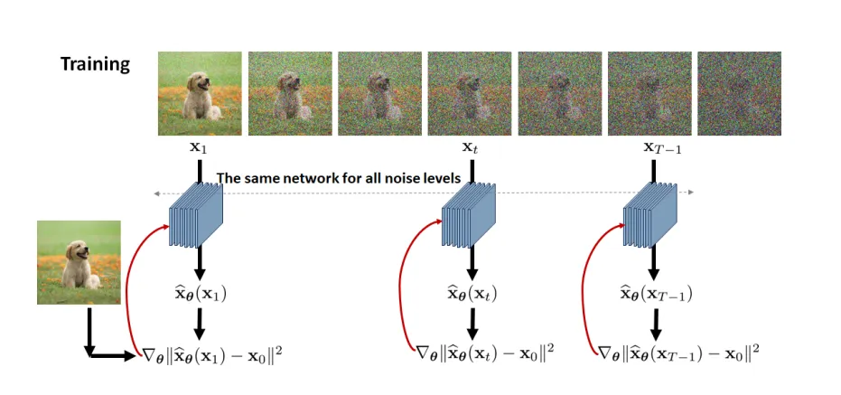
ELBO θ ( x ) = E q ( x 1 ∣ x 0 ) [ log p θ ( x 0 ∣ x 1 ) ] − D K L ( q ( x T ∣ x 0 ) ∥ p ( x T ) ) ⏟ nothing to train − ∑ t = 2 T E q ( x t ∣ x 0 ) [ 1 2 σ q 2 ( t ) ∥ μ q ( x t , x 0 ) − μ θ ( x t ) ∥ 2 ] . \begin{aligned}\operatorname{ELBO}_{\boldsymbol{\theta}}(\mathbf{x})&=\mathbb{E}_{q(\mathbf{x}_1|\mathbf{x}_0)}[\log p_{\boldsymbol{\theta}}(\mathbf{x}_0|\mathbf{x}_1)]-\underbrace{\mathbb{D}_{\mathrm{KL}}\left(q(\mathbf{x}_T|\mathbf{x}_0)\|p(\mathbf{x}_T)\right)}_{\text{nothing to train}}\\&-\sum_{t=2}^T\mathbb{E}_{q(\mathbf{x}_t|\mathbf{x}_0)}\bigg[\frac1{2\sigma_q^2(t)}\|\boldsymbol{\mu}_q(\mathbf{x}_t,\mathbf{x}_0)-\boldsymbol{\mu}_{\boldsymbol{\theta}}(\mathbf{x}_t)\|^2\bigg].\end{aligned} ELBO θ ( x ) = E q ( x 1 ∣ x 0 ) [ log p θ ( x 0 ∣ x 1 )] − nothing to train D KL ( q ( x T ∣ x 0 ) ∥ p ( x T ) ) − t = 2 ∑ T E q ( x t ∣ x 0 ) [ 2 σ q 2 ( t ) 1 ∥ μ q ( x t , x 0 ) − μ θ ( x t ) ∥ 2 ] . Given x t ∼ q ( x t ∣ x 0 ) \mathbf{x}_t\sim q(\mathbf{x}_t|\mathbf{x}_0) x t ∼ q ( x t ∣ x 0 ) log p θ ( x 0 ∣ x 1 ) \log p_{\boldsymbol{\theta}}(\mathbf{x}_0|\mathbf{x}_1) log p θ ( x 0 ∣ x 1 ) log N ( x 0 ∣ μ θ ( x 1 ) , σ q 2 ( 1 ) I ) . \log\mathcal{N}(\mathbf{x}_0|\boldsymbol{\mu}_{\boldsymbol{\theta}}(\mathbf{x}_1),\sigma_q^2(1)\mathbf{I}). log N ( x 0 ∣ μ θ ( x 1 ) , σ q 2 ( 1 ) I ) . x 1 \mathbf{x}_1 x 1 μ θ ( x 1 ) \boldsymbol\mu_{\theta}(\mathbf{x}_1) μ θ ( x 1 ) 7 Training and Inference# The ELBO suggests that we need to find a network μ θ \boldsymbol{\mu_\mathrm{\theta}} μ θ
1 2 σ q 2 ( t ) ∥ μ q ( x t , x 0 ) ⏟ known − μ θ ( x t ) ⏟ network ∥ 2 . \frac1{2\sigma_q^2(t)}\|\underbrace{\boldsymbol{\mu}_q(\mathbf{x}_t,\mathbf{x}_0)}_{\text{known}}-\underbrace{\boldsymbol{\mu}_{\boldsymbol{\theta}}(\mathbf{x}_t)}_{\text{network}}\|^2. 2 σ q 2 ( t ) 1 ∥ known μ q ( x t , x 0 ) − network μ θ ( x t ) ∥ 2 . We recall that
μ q ( x t , x 0 ) = ( 1 − α ‾ t − 1 ) α t 1 − α ‾ t x t + ( 1 − α t ) α ‾ t − 1 1 − α ‾ t x 0 . \boldsymbol{\mu}_q(\mathbf{x}_t,\mathbf{x}_0)=\frac{(1-\overline{\alpha}_{t-1})\sqrt{\alpha_t}}{1-\overline{\alpha}_t}\mathbf{x}_t+\frac{(1-\alpha_t)\sqrt{\overline{\alpha}_{t-1}}}{1-\overline{\alpha}_t}\mathbf{x}_0. μ q ( x t , x 0 ) = 1 − α t ( 1 − α t − 1 ) α t x t + 1 − α t ( 1 − α t ) α t − 1 x 0 . Since μ θ \boldsymbol{\mu_{\theta}} μ θ d e s i g n design d es i g n
μ θ ⏟ a n e t w o r k ( x t ) = d e f ( 1 − α ‾ t − 1 ) α t 1 − α ‾ t x t + ( 1 − α t ) α ‾ t − 1 1 − α ‾ t x ^ θ ( x t ) ⏟ a n o t h e r n e t w o r k . \underbrace{\boldsymbol{\mu_{\theta}}}_{\mathrm{a~network}}(\mathbf{x}_{t})\stackrel{\mathrm{def}}{=}\frac{(1-\overline{\alpha}_{t-1})\sqrt{\alpha_{t}}}{1-\overline{\alpha}_{t}}\mathbf{x}_{t}+\frac{(1-\alpha_{t})\sqrt{\overline{\alpha}_{t-1}}}{1-\overline{\alpha}_{t}}\underbrace{\widehat{\mathbf{x}}_{\boldsymbol{\theta}}(\mathbf{x}_{t})}_{\mathrm{another~network}}\:. a network μ θ ( x t ) = def 1 − α t ( 1 − α t − 1 ) α t x t + 1 − α t ( 1 − α t ) α t − 1 another network x θ ( x t ) . Then we have
1 2 σ q 2 ( t ) ∥ μ q ( x t , x 0 ) − μ θ ( x t ) ∥ 2 = 1 2 σ q 2 ( t ) ∥ ( 1 − α t ) α ‾ t − 1 1 − α ‾ t ( x ^ θ ( x t ) − x 0 ) ∥ 2 = 1 2 σ q 2 ( t ) ( 1 − α t ) 2 α ‾ t − 1 ( 1 − α ‾ t ) 2 ∥ x ^ θ ( x t ) − x 0 ∥ 2 \begin{aligned}\frac{1}{2\sigma_{q}^{2}(t)}\|\boldsymbol{\mu}_{q}(\mathbf{x}_{t},\mathbf{x}_{0})-\boldsymbol{\mu}_{\boldsymbol{\theta}}(\mathbf{x}_{t})\|^{2}&=\frac{1}{2\sigma_{q}^{2}(t)}\left\|\frac{(1-\alpha_{t})\sqrt{\overline{\alpha}_{t-1}}}{1-\overline{\alpha}_{t}}(\widehat{\mathbf{x}}_{\boldsymbol{\theta}}(\mathbf{x}_{t})-\mathbf{x}_{0})\right\|^{2}\\&=\frac1{2\sigma_q^2(t)}\frac{(1-\alpha_t)^2\overline{\alpha}_{t-1}}{(1-\overline{\alpha}_t)^2}\left\|\widehat{\mathbf{x}}_{\boldsymbol{\theta}}(\mathbf{x}_t)-\mathbf{x}_0\right\|^2\end{aligned} 2 σ q 2 ( t ) 1 ∥ μ q ( x t , x 0 ) − μ θ ( x t ) ∥ 2 = 2 σ q 2 ( t ) 1 1 − α t ( 1 − α t ) α t − 1 ( x θ ( x t ) − x 0 ) 2 = 2 σ q 2 ( t ) 1 ( 1 − α t ) 2 ( 1 − α t ) 2 α t − 1 ∥ x θ ( x t ) − x 0 ∥ 2 Therefore ELBO can be simplified into
E L B O θ = E q ( x 1 ∣ x 0 ) [ log p θ ( x 0 ∣ x 1 ) ] − ∑ t = 2 T E q ( x t ∣ x 0 ) [ 1 2 σ q 2 ( t ) ∥ μ q ( x t , x 0 ) − μ θ ( x t ) ∥ 2 ] = E q ( x 1 ∣ x 0 ) [ log p θ ( x 0 ∣ x 1 ) ] − ∑ t = 2 T E q ( x t ∣ x 0 ) [ 1 2 σ q 2 ( t ) ( 1 − α t ) 2 α ‾ t − 1 ( 1 − α ‾ t ) 2 ∥ x ^ θ ( x t ) − x 0 ∥ 2 ] . \begin{aligned} \mathrm{ELBO}_{\boldsymbol{\theta}}& =\mathbb{E}_{q(\mathbf{x}_1|\mathbf{x}_0)}[\log p_{\boldsymbol{\theta}}(\mathbf{x}_0|\mathbf{x}_1)]-\sum_{t=2}^T\mathbb{E}_{q(\mathbf{x}_t|\mathbf{x}_0)}\Big[\frac1{2\sigma_q^2(t)}\|\boldsymbol{\mu}_q(\mathbf{x}_t,\mathbf{x}_0)-\boldsymbol{\mu}_{\boldsymbol{\theta}}(\mathbf{x}_t)\|^2\Big] \\ &=\mathbb{E}_{q(\mathbf{x}_1|\mathbf{x}_0)}[\log p_{\boldsymbol{\theta}}(\mathbf{x}_0|\mathbf{x}_1)]-\sum_{t=2}^T\mathbb{E}_{q(\mathbf{x}_t|\mathbf{x}_0)}\Big[\frac1{2\sigma_q^2(t)}\frac{(1-\alpha_t)^2\overline{\alpha}_{t-1}}{(1-\overline{\alpha}_t)^2}\left\|\widehat{\mathbf{x}}_{\boldsymbol{\theta}}(\mathbf{x}_t)-\mathbf{x}_0\right\|^2\Big]. \end{aligned} ELBO θ = E q ( x 1 ∣ x 0 ) [ log p θ ( x 0 ∣ x 1 )] − t = 2 ∑ T E q ( x t ∣ x 0 ) [ 2 σ q 2 ( t ) 1 ∥ μ q ( x t , x 0 ) − μ θ ( x t ) ∥ 2 ] = E q ( x 1 ∣ x 0 ) [ log p θ ( x 0 ∣ x 1 )] − t = 2 ∑ T E q ( x t ∣ x 0 ) [ 2 σ q 2 ( t ) 1 ( 1 − α t ) 2 ( 1 − α t ) 2 α t − 1 ∥ x θ ( x t ) − x 0 ∥ 2 ] . The first term is
log p θ ( x 0 ∣ x 1 ) = log N ( x 0 ∣ μ θ ( x 1 ) , σ q 2 ( 1 ) I ) ∝ − 1 2 σ q 2 ( 1 ) ∥ μ θ ( x 1 ) − x 0 ∥ 2 definition = − 1 2 σ q 2 ( 1 ) ∥ ( 1 − α ‾ 0 ) α 1 1 − α ‾ 1 x 1 + ( 1 − α 1 ) α ‾ 0 1 − α ‾ 1 x ^ θ ( x 1 ) − x 0 ∥ 2 r e c a l l α 0 = 1 = − 1 2 σ q 2 ( 1 ) ∥ ( 1 − α 1 ) 1 − α ‾ 1 x ^ θ ( x 1 ) − x 0 ∥ 2 = − 1 2 σ q 2 ( 1 ) ∥ x ^ θ ( x 1 ) − x 0 ∥ 2 r e c a l l α ‾ 1 = α 1 \begin{aligned} \\ \log p_{\boldsymbol{\theta}}(\mathbf{x}_0|\mathbf{x}_1)& =\log\mathcal{N}(\mathbf{x}_0|\boldsymbol{\mu}_{\boldsymbol{\theta}}(\mathbf{x}_1),\sigma_q^2(1)\mathbf{I})\propto-\frac{1}{2\sigma_q^2(1)}\|\boldsymbol{\mu}_{\boldsymbol{\theta}}(\mathbf{x}_1)-\mathbf{x}_0\|^2 && \text{definition} \\ &=-\frac{1}{2\sigma_q^2(1)}\left\|\frac{(1-\overline{\alpha}_0)\sqrt{\alpha_1}}{1-\overline{\alpha}_1}\mathbf{x}_1+\frac{(1-\alpha_1)\sqrt{\overline{\alpha}_0}}{1-\overline{\alpha}_1}\widehat{\mathbf{x}}_{\boldsymbol{\theta}}(\mathbf{x}_1)-\mathbf{x}_0\right\|^2&& \mathrm{recall~}\alpha_{0}=1 \\ &=-\frac{1}{2\sigma_{q}^{2}(1)}\left\|\frac{(1-\alpha_{1})}{1-\overline{\alpha}_{1}}\widehat{\mathbf{x}}_{\boldsymbol{\theta}}(\mathbf{x}_{1})-\mathbf{x}_{0}\right\|^{2}=-\frac{1}{2\sigma_{q}^{2}(1)}\left\|\widehat{\mathbf{x}}_{\boldsymbol{\theta}}(\mathbf{x}_{1})-\mathbf{x}_{0}\right\|^{2}\quad\mathrm{recall~}\overline{\alpha}_{1}=\alpha_{1} \\ \end{aligned} log p θ ( x 0 ∣ x 1 ) = log N ( x 0 ∣ μ θ ( x 1 ) , σ q 2 ( 1 ) I ) ∝ − 2 σ q 2 ( 1 ) 1 ∥ μ θ ( x 1 ) − x 0 ∥ 2 = − 2 σ q 2 ( 1 ) 1 1 − α 1 ( 1 − α 0 ) α 1 x 1 + 1 − α 1 ( 1 − α 1 ) α 0 x θ ( x 1 ) − x 0 2 = − 2 σ q 2 ( 1 ) 1 1 − α 1 ( 1 − α 1 ) x θ ( x 1 ) − x 0 2 = − 2 σ q 2 ( 1 ) 1 ∥ x θ ( x 1 ) − x 0 ∥ 2 recall α 1 = α 1 definition recall α 0 = 1 Then ELBO will be
E L B O θ = − ∑ t = 1 T E q ( x t ∣ x 0 ) [ 1 2 σ q 2 ( t ) ( 1 − α t ) 2 α ‾ t − 1 ( 1 − α ‾ t ) 2 ∥ x ^ θ ( x t ) − x 0 ∥ 2 ] . \begin{aligned} &\mathrm{ELBO}_{\boldsymbol{\theta}}=-\sum_{t=1}^T\mathbb{E}_{q(\mathbf{x}_t|\mathbf{x}_0)}\Big[\frac{1}{2\sigma_q^2(t)}\frac{(1-\alpha_t)^2\overline{\alpha}_{t-1}}{(1-\overline{\alpha}_t)^2}\left\|\widehat{\mathbf{x}}_{\boldsymbol{\theta}}(\mathbf{x}_t)-\mathbf{x}_0\right\|^2\Big]. \end{aligned} ELBO θ = − t = 1 ∑ T E q ( x t ∣ x 0 ) [ 2 σ q 2 ( t ) 1 ( 1 − α t ) 2 ( 1 − α t ) 2 α t − 1 ∥ x θ ( x t ) − x 0 ∥ 2 ] . Therefore, the training of the neural network boils down to a simple loss function:
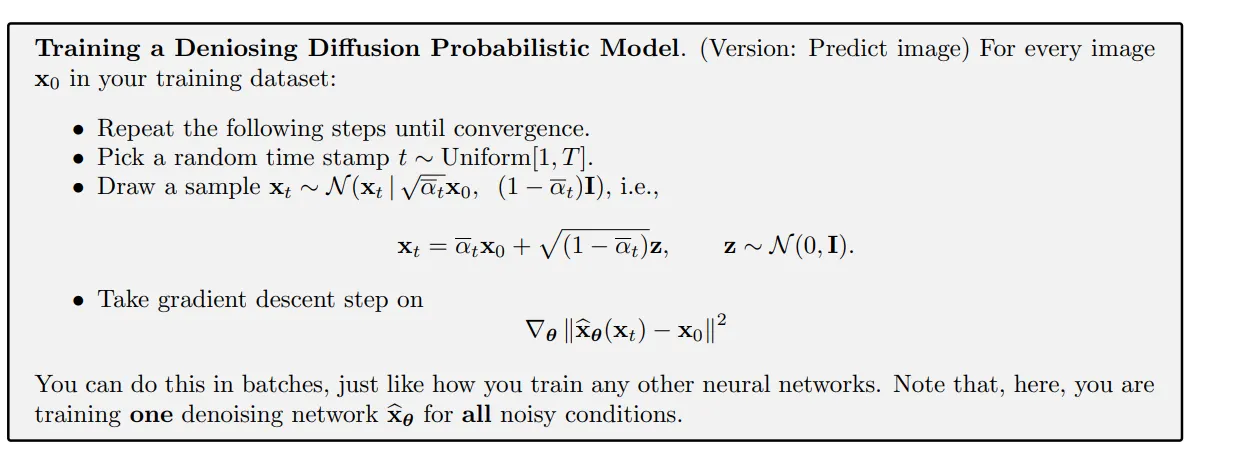
The loss function for a denoising diffusion probabilistic model:
θ ∗ = argmin θ ∑ t = 1 T 1 2 σ q 2 ( t ) ( 1 − α t ) 2 α ‾ t − 1 ( 1 − α ‾ t ) 2 E q ( x t ∣ x 0 ) [ ∥ x ^ θ ( x t ) − x 0 ∥ 2 ] . \boldsymbol{\theta}^*=\underset{\boldsymbol{\theta}}{\operatorname*{argmin}}\sum_{t=1}^T\frac1{2\sigma_q^2(t)}\frac{(1-\alpha_t)^2\overline{\alpha}_{t-1}}{(1-\overline{\alpha}_t)^2}\mathbb{E}_{q(\mathbf{x}_t|\mathbf{x}_0)}\bigg[\left\|\widehat{\mathbf{x}}_{\boldsymbol{\theta}}(\mathbf{x}_t)-\mathbf{x}_0\right\|^2\bigg]. θ ∗ = θ argmin t = 1 ∑ T 2 σ q 2 ( t ) 1 ( 1 − α t ) 2 ( 1 − α t ) 2 α t − 1 E q ( x t ∣ x 0 ) [ ∥ x θ ( x t ) − x 0 ∥ 2 ] .
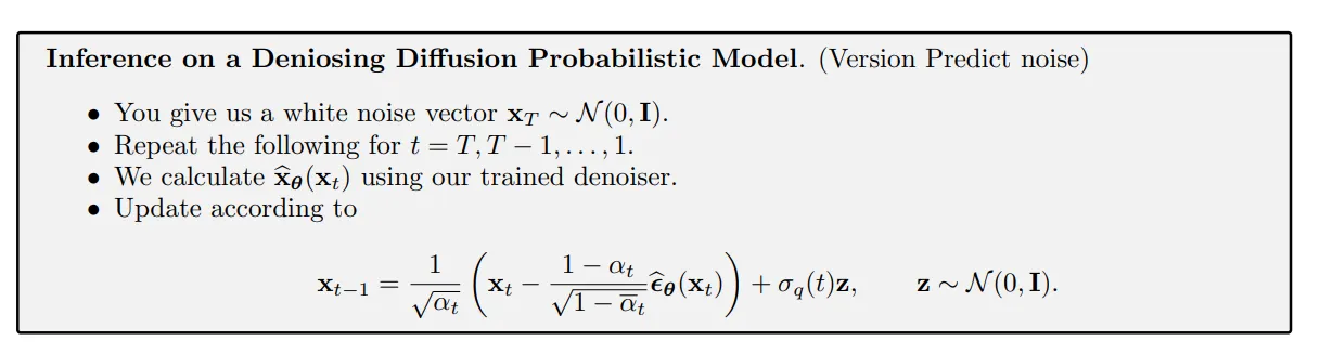
Inference: recursively
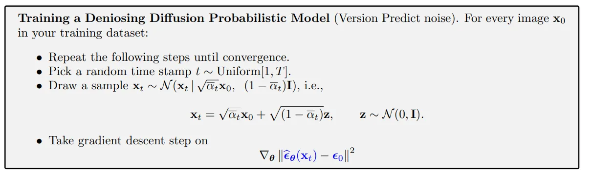
8 Derivation based on Noise Vector# We can show that
μ q ( x t , x 0 ) = 1 α t x t − 1 − α t 1 − α ‾ t α t ϵ 0 . \begin{aligned} \boldsymbol{\mu}_q(\mathbf{x}_t,\mathbf{x}_0) =\frac1{\sqrt{\alpha_t}}\mathbf{x}_t-\frac{1-\alpha_t}{\sqrt{1-\overline{\alpha}_t}\sqrt{\alpha}_t}\boldsymbol{\epsilon}_0. \end{aligned} μ q ( x t , x 0 ) = α t 1 x t − 1 − α t α t 1 − α t ϵ 0 . So we can design our mean estimator μ θ \boldsymbol{\mu_{\theta}} μ θ
μ θ ( x t ) = 1 α t x t − 1 − α t 1 − α ‾ t α t ϵ ^ θ ( x t ) . \boldsymbol{\mu}_{\boldsymbol{\theta}}(\mathbf{x}_t)=\frac{1}{\sqrt{\alpha_t}}\mathbf{x}_t-\frac{1-\alpha_t}{\sqrt{1-\overline{\alpha}_t}\sqrt{\alpha}_t}\widehat{\boldsymbol{\epsilon}}_{\boldsymbol{\theta}}(\mathbf{x}_t). μ θ ( x t ) = α t 1 x t − 1 − α t α t 1 − α t ϵ θ ( x t ) . Then we can get a new ELBO
E L B O θ = − ∑ t = 1 T E q ( x t ∣ x 0 ) [ 1 2 σ q 2 ( t ) ( 1 − α t ) 2 α ‾ t − 1 ( 1 − α ‾ t ) 2 ∥ ϵ ^ θ ( x t ) − ϵ 0 ∥ 2 ] . \mathrm{ELBO}_{\boldsymbol{\theta}}=-\sum_{t=1}^T\mathbb{E}_{q(\mathbf{x}_t|\mathbf{x}_0)}\Big[\frac{1}{2\sigma_q^2(t)}\frac{(1-\alpha_t)^2\overline{\alpha}_{t-1}}{(1-\overline{\alpha}_t)^2}\left\|\widehat{\boldsymbol{\epsilon}}_{\boldsymbol{\theta}}(\mathbf{x}_t)-\boldsymbol{\epsilon}_0\right\|^2\Big]. ELBO θ = − t = 1 ∑ T E q ( x t ∣ x 0 ) [ 2 σ q 2 ( t ) 1 ( 1 − α t ) 2 ( 1 − α t ) 2 α t − 1 ∥ ϵ θ ( x t ) − ϵ 0 ∥ 2 ] .
x t − 1 ∼ p θ ( x t − 1 ∣ x t ) = N ( x t − 1 ∣ μ θ ( x t ) , σ q 2 ( t ) I ) = μ θ ( x t ) + σ q 2 ( t ) z = 1 α t x t − 1 − α t 1 − α ‾ t α t ϵ ^ θ ( x t ) + σ q ( t ) z = 1 α t ( x t − 1 − α t 1 − α ‾ t ϵ ^ θ ( x t ) ) + σ q ( t ) z \begin{aligned} \mathbf{x}_{t-1}\sim p_{\boldsymbol{\theta}}(\mathbf{x}_{t-1}\mid\mathbf{x}_{t})& =\mathcal{N}(\mathbf{x}_{t-1}\mid\boldsymbol{\mu}_{\boldsymbol{\theta}}(\mathbf{x}_t),\sigma_q^2(t)\mathbf{I}) \\ &=\mu_{\boldsymbol{\theta}}(\mathbf{x}_t)+\sigma_q^2(t)\mathbf{z} \\ &=\frac{1}{\sqrt{\alpha_{t}}}\mathbf{x}_{t}-\frac{1-\alpha_{t}}{\sqrt{1-\overline{\alpha}_{t}}\sqrt{\alpha}_{t}}\widehat{\boldsymbol{\epsilon}}_{\boldsymbol{\theta}}(\mathbf{x}_{t})+\sigma_{q}(t)\mathbf{z} \\ &=\frac1{\sqrt{\alpha_t}}\left(\mathbf{x}_t-\frac{1-\alpha_t}{\sqrt{1-\overline{\alpha}_t}}\widehat{\boldsymbol{\epsilon}}_{\boldsymbol{\theta}}(\mathbf{x}_t)\right)+\sigma_q(t)\mathbf{z} \end{aligned} x t − 1 ∼ p θ ( x t − 1 ∣ x t ) = N ( x t − 1 ∣ μ θ ( x t ) , σ q 2 ( t ) I ) = μ θ ( x t ) + σ q 2 ( t ) z = α t 1 x t − 1 − α t α t 1 − α t ϵ θ ( x t ) + σ q ( t ) z = α t 1 ( x t − 1 − α t 1 − α t ϵ θ ( x t ) ) + σ q ( t ) z So we have
Reference# [1] Chan, Stanley H. “Tutorial on Diffusion Models for Imaging and Vision.” arXiv preprint arXiv:2403.18103 (2024).


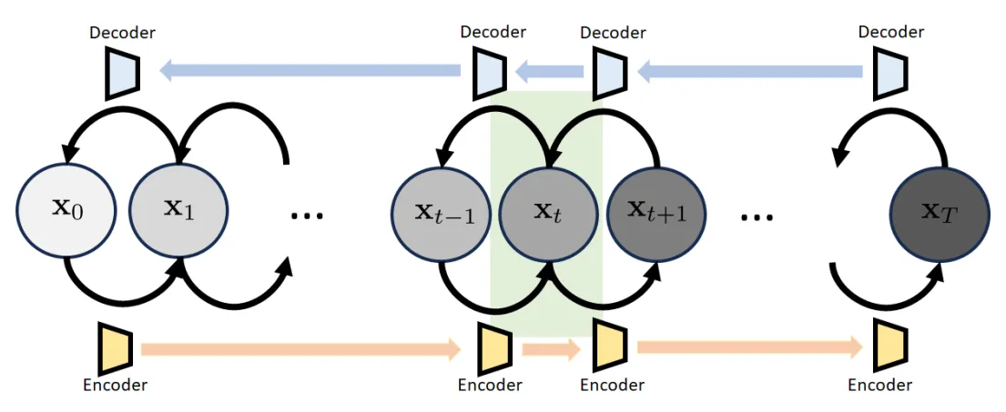 It is called the variational diffusion model. The variational diffusion model has a sequence of states :
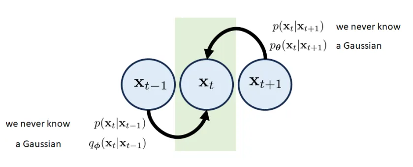

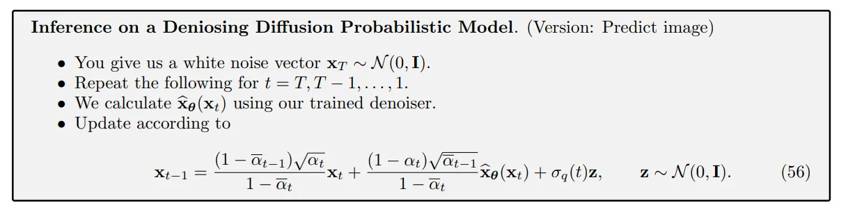 Consequently, the inference step can be derived through