Policy Gradient Methods

Policies can be represented by parameterized functions denoted as $π(a|s, θ)$ , where $θ\in \mathbb{R}^{m}$ is a parameter vector.

When policies are represented as functions, optimal policies can be obtained by optimizing certain scalar metrics. Such a method is called policy gradient.

9.1 Policy representation: From table to function#

how to define optimal policies? maximize every state value. maximize certain scalar metrics.
how to update a policy? changing the entries in the table; changing the parameter $θ$ .
how to retrieve the probability of an action? looking up the corresponding entry in the table;

Suppose that $J(\theta)$ is a scalar metric. Then optimal policies can be obtained by

\theta_{t+1}=\theta_t+\alpha\nabla_\theta J(\theta_t)

where $\nabla_{\theta}J$ is the gradient of $J$ with respect to $θ$ , $t$ is the time step, and $α$ is the optimization rate.

9.2 Metrics for defining optimal policies#

Metric 1: Average state value#

\bar{v}_\pi=\sum_{s\in\mathcal{S}}d(s)v_\pi(s),

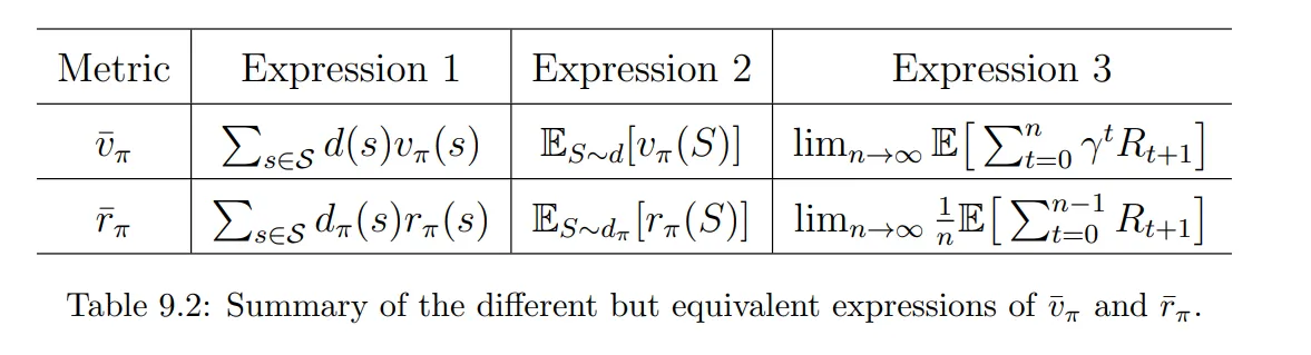
where $d(s)$ is the weight of state $s.$ It satisfies $d(s)\geq0$ for any $s\in\mathcal{S}$ and $\sum_s\in\mathcal{S}d(s)=1.$ Therefore, we can interpret $d(s)$ as a probability distribution of $s.$ Then, the metric can be written as

\bar{v}_\pi=\mathbb{E}_{S\sim d}[v_\pi(S)].

How to select the distribution $d$ ?#

$d$ $d$ is independent of the policy $\pi$ $π$ .
- Treat all the states equally important and select $d_0(s)=$ $1/|\mathcal{S}|.$
- We are only interested in a specific state $s_0$ (e.g., the agent always starts from $s_0).$ In this case, we can design $d_0(s_0)=1,\quad d_0(s\neq s_0)=0.$
$d$ is dependent on the policy $\pi$ . it is common to select $d$ as $d_\pi$ , which is the stationary distribution under $\pi$ . One basic property of $d_\pi$ is that it satisfies $d_\pi^TP_\pi=d_\pi^T,$ where $P_\pi$ is the state transition probability matrix.

two important equivalent expressions of $\overline{v}_{\pi}$ .#

First one

J(\theta)=\lim_{n\to\infty}\mathbb{E}\left[\sum_{t=0}^n\gamma^tR_{t+1}\right]=\mathbb{E}\left[\sum_{t=0}^\infty\gamma^tR_{t+1}\right].

Which is easy to show:

\begin{aligned} \mathbb{E}\left[\sum_{t=0}^\infty\gamma^tR_{t+1}\right]& \begin{aligned}=\sum_{s\in\mathcal{S}}d(s)\mathbb{E}\left[\sum_{t=0}^\infty\gamma^tR_{t+1}|S_0=s\right]\end{aligned} \\ &=\sum_{s\in\mathcal{S}}d(s)v_\pi(s) \\ &=\bar{v}_{\pi}. \end{aligned}

Second one

\overline{v}_{\pi}=d^{T}v_{\pi}.

Metric 2: Average reward#

\begin{aligned}\bar{r}_{\pi}&\doteq\sum_{s\in\mathcal{S}}d_\pi(s)r_\pi(s)\\&=\mathbb{E}_{S\sim d_\pi}[r_\pi(S)],\end{aligned}

where $d_{\pi}$ is the stationary distribution and

r_\pi(s)\doteq\sum_{a\in\mathcal{A}}\pi(a|s,\theta)r(s,a)=\mathbb{E}_{A\sim\pi(s,\theta)}[r(s,A)|s]

is the expectation of the immediate rewards. Here, $r(s,a)\doteq\mathbb{E}[R|s,a]=\sum_rrp(r|s,a)$ .

two important equivalent expressions of $\overline{r}_{\pi}$ #

First one

J(\theta)=\lim_{n\to\infty}\frac1n\mathbb{E}\left[\sum_{t=0}^{n-1}R_{t+1}\right].

It is easy to show that

\lim_{n\to\infty}\frac{1}{n}\mathbb{E}\left[\sum_{t=0}^{n-1}R_{t+1}\right]=\sum_{s\in\mathcal{S}}d_\pi(s)r_\pi(s)=\bar{r}_\pi.

Second one

\bar{r}_\pi=\sum_{s\in\mathcal{S}}d_\pi(s)r_\pi(s)=d_\pi^Tr_\pi.

Summary#

RL9-1

The two metrics $\bar{v}_\pi$ and $\bar{r}_\pi$ are equivalent in the discounted case where $\gamma<1.$ In particular, it can be shown that

\bar{r}_\pi=(1-\gamma)\bar{v}_\pi.

9.3 Gradients of the metrics#

9.4 Monte Carlo policy gradient (REINFORCE)#

The gradient-ascent algorithm for maximizing $J(\theta)$ is

\begin{aligned}\theta_{t+1}&=\theta_t+\alpha\nabla_\theta J(\theta_t)\\&=\theta_t+\alpha\mathbb{E}\Big[\nabla_\theta\ln\pi(A|S,\theta_t)q_\pi(S,A)\Big],\end{aligned}

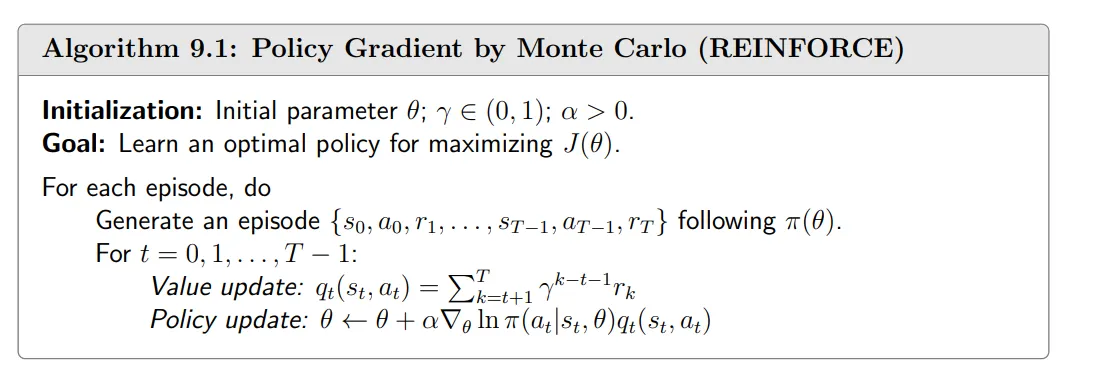
where $\alpha>0$ is a constant learning rate. Since the true gradient is unknown, we can replace the true gradient with a stochastic gradient to obtain the following algorithm:

\theta_{t+1}=\theta_t+\alpha\nabla_\theta\ln\pi(a_t|s_t,\theta_t)q_t(s_t,a_t),

where $q_t(s_t,a_t)$ is an approximation of $q_\pi(s_t,a_t).$ If $q_t(s_t,a_t)$ is obtained by Monte Carlo estimation, the algorithm is called REINFORCE or Monte Carlo policy gradient which is one of earliest and simplest policy gradient algorithms.

Since $\nabla_\theta\ln\pi(a_t|s_t,\theta_t)=\frac{\nabla_\theta\pi(a_t|s_t,\theta_t)}{\pi(a_t|s_t,\theta_t)}$ , we have

\theta_{t+1}=\theta_t+\alpha\underbrace{\left(\frac{q_t(s_t,a_t)}{\pi(a_t|s_t,\theta_t)}\right)}_{\beta_t}\nabla_\theta\pi(a_t|s_t,\theta_t),

Which can be further written concisely as

\theta_{t+1}=\theta_t+\alpha\beta_t\nabla_\theta\pi(a_t|s_t,\theta_t).

It is clear that $\pi(a_t|s_t,\theta_{t+1})\geq\pi(a_t|s_t,\theta_t)$ when $\beta_t\geq0$ and $\pi(a_t|s_t,\theta_{t+1})<\pi(a_t|s_t,\theta_t)$ when $\beta_t<0$ .

Unfortunately, the ideal ways for sampling S and A are not strictly followed in practice due to their low efficiency of sample usage. A more sample-efficient implementation is given RL9-1