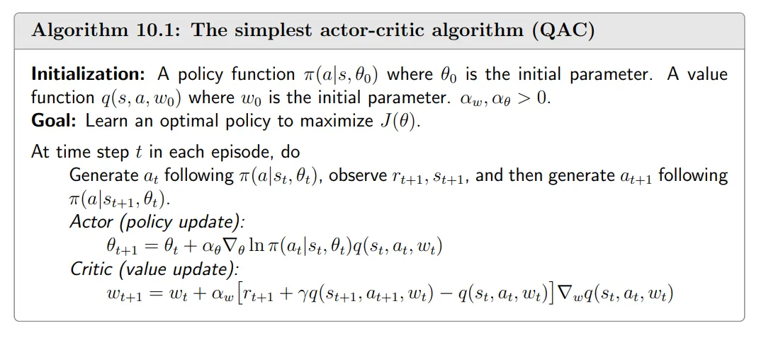
“actor-critic” refers to a structure that incorporates both policy-based and value-based methods. An “actor” refers to a policy update step. An “critic” refers to a value update step. 10.1 The simplest actor-critic algorithm (QAC)# The gradient-ascent algorithm for maximizing J ( θ ) J(θ) J ( θ )
θ t + 1 = θ t + α ∇ θ J ( θ t ) = θ t + α E S ∼ η , A ∼ π [ ∇ θ ln π ( A ∣ S , θ t ) q π ( S , A ) ] , \begin{aligned} \theta_{t+1}& =\theta_t+\alpha\nabla_\theta J(\theta_t) \\ &=\theta_t+\alpha\mathbb{E}_{S\sim\eta,A\sim\pi}\Big[\nabla_\theta\ln\pi(A|S,\theta_t)q_\pi(S,A)\Big], \end{aligned} θ t + 1 = θ t + α ∇ θ J ( θ t ) = θ t + α E S ∼ η , A ∼ π [ ∇ θ ln π ( A ∣ S , θ t ) q π ( S , A ) ] , where η η η
θ t + 1 = θ t + α ∇ θ ln π ( a t ∣ s t , θ t ) q t ( s t , a t ) . \theta_{t+1}=\theta_t+\alpha\nabla_\theta\ln\pi(a_t|s_t,\theta_t)q_t(s_t,a_t). θ t + 1 = θ t + α ∇ θ ln π ( a t ∣ s t , θ t ) q t ( s t , a t ) . If q t ( s t , a t ) q_t(s_t,a_t) q t ( s t , a t ) REINFORCE or Monte Carlo policy gradient . If q t ( s t , a t ) q_t(s_t,a_t) q t ( s t , a t ) actor-critic . Therefore, actor-critic methods can be obtained by incorporating TD-based value estimation into policy gradient methods. The critic corresponds to the value update step via the Sarsa algorithm. This actor-citric algorithm is sometimes called Q Q Q actor-critic (QAC).
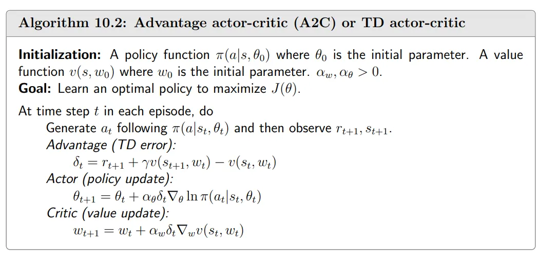
10.2 Advantage actor-critic (A2C)# The core idea of this algorithm is to introduce a baseline to reduce estimation variance .
Baseline invariance# One interesting property of the policy gradient is that it is invariant to an additional baseline .
E S ∼ η , A ∼ π [ ∇ θ ln π ( A ∣ S , θ t ) q π ( S , A ) ] = E S ∼ η , A ∼ π [ ∇ θ ln π ( A ∣ S , θ t ) ( q π ( S , A ) − b ( S ) ) ] , \mathbb{E}_{S\sim\eta,A\sim\pi}\Big[\nabla_\theta\ln\pi(A|S,\theta_t)q_\pi(S,A)\Big]=\mathbb{E}_{S\sim\eta,A\sim\pi}\Big[\nabla_\theta\ln\pi(A|S,\theta_t)(q_\pi(S,A)-b(S))\Big], E S ∼ η , A ∼ π [ ∇ θ ln π ( A ∣ S , θ t ) q π ( S , A ) ] = E S ∼ η , A ∼ π [ ∇ θ ln π ( A ∣ S , θ t ) ( q π ( S , A ) − b ( S )) ] , where the additional baseline b ( S ) b(S) b ( S ) S S S
Why useful? It can reduce the approximation variance when we use samples to approximate the true gradient.
X ( S , A ) ≐ ∇ θ ln π ( A ∣ S , θ t ) [ q π ( S , A ) − b ( S ) ] X(S,A)\doteq\nabla_\theta\ln\pi(A|S,\theta_t)[q_\pi(S,A)-b(S)] X ( S , A ) ≐ ∇ θ ln π ( A ∣ S , θ t ) [ q π ( S , A ) − b ( S )] Then, the true gradient is E [ X ( S , A ) ] \mathbb{E}[X(S, A)] E [ X ( S , A )] var ( X ) \text{var}(X) var ( X )
Optimal baseline that minimizes variance:
b ∗ ( s ) = E A ∼ π [ ∥ ∇ θ ln π ( A ∥ s , θ t ) ∥ 2 q π ( s , A ) ] E A ∼ π [ ∥ ∇ θ ln π ( A ∣ s , θ t ) ∥ 2 ] , s ∈ S b^*(s)=\frac{\mathbb{E}_{A\sim\pi}\big[\|\nabla_\theta\ln\pi(A\|s,\theta_t)\|^2q_\pi(s,A)\big]}{\mathbb{E}_{A\sim\pi}\big[\|\nabla_\theta\ln\pi(A|s,\theta_t)\|^2\big]},\quad s\in\mathcal{S} b ∗ ( s ) = E A ∼ π [ ∥ ∇ θ ln π ( A ∣ s , θ t ) ∥ 2 ] E A ∼ π [ ∥ ∇ θ ln π ( A ∥ s , θ t ) ∥ 2 q π ( s , A ) ] , s ∈ S Suboptimal baseline (simpler):
b † ( s ) = E A ∼ π [ q π ( s , A ) ] = v π ( s ) , s ∈ S . b^\dagger(s)=\mathbb{E}_{A\sim\pi}[q_\pi(s,A)]=v_\pi(s),\quad s\in\mathcal{S}. b † ( s ) = E A ∼ π [ q π ( s , A )] = v π ( s ) , s ∈ S . which is the state value.
Algorithm description# When b ( s ) = v π ( s ) b(s) = v_{\pi}(s) b ( s ) = v π ( s )
θ t + 1 = θ t + α E [ ∇ θ ln π ( A ∣ S , θ t ) [ q π ( S , A ) − v π ( S ) ] ] ≐ θ t + α E [ ∇ θ ln π ( A ∣ S , θ t ) δ π ( S , A ) ] . \begin{gathered} \theta_{t+1} =\theta_t+\alpha\mathbb{E}\Big[\nabla_\theta\ln\pi(A|S,\theta_t)[q_\pi(S,A)-v_\pi(S)]\Big] \\ \doteq\theta_t+\alpha\mathbb{E}\bigg[\nabla_\theta\ln\pi(A|S,\theta_t)\delta_\pi(S,A)\bigg]. \end{gathered} θ t + 1 = θ t + α E [ ∇ θ ln π ( A ∣ S , θ t ) [ q π ( S , A ) − v π ( S )] ] ≐ θ t + α E [ ∇ θ ln π ( A ∣ S , θ t ) δ π ( S , A ) ] . Here,
δ π ( S , A ) ≐ q π ( S , A ) − v π ( S ) \delta_\pi(S,A)\doteq q_\pi(S,A)-v_\pi(S) δ π ( S , A ) ≐ q π ( S , A ) − v π ( S ) is called the advantage function .
The stochastic version is
θ t + 1 = θ t + α ∇ θ ln π ( a t ∣ s t , θ t ) [ q t ( s t , a t ) − v t ( s t ) ] = θ t + α ∇ θ ln π ( a t ∣ s t , θ t ) δ t ( s t , a t ) , \theta_{t+1}=\theta_t+\alpha\nabla_\theta\ln\pi(a_t|s_t,\theta_t)[q_t(s_t,a_t)-v_t(s_t)]\\=\theta_t+\alpha\nabla_\theta\ln\pi(a_t|s_t,\theta_t)\delta_t(s_t,a_t), θ t + 1 = θ t + α ∇ θ ln π ( a t ∣ s t , θ t ) [ q t ( s t , a t ) − v t ( s t )] = θ t + α ∇ θ ln π ( a t ∣ s t , θ t ) δ t ( s t , a t ) , where s t s_{t} s t a t a_{t} a t S S S A A A t t t
The algorithm is as follows:
The advantage function is approximated by the TD error:
q t ( s t , a t ) − v t ( s t ) ≈ r t + 1 + γ v t ( s t + 1 ) − v t ( s t ) . q_t(s_t,a_t)-v_t(s_t)\approx r_{t+1}+\gamma v_t(s_{t+1})-v_t(s_t). q t ( s t , a t ) − v t ( s t ) ≈ r t + 1 + γ v t ( s t + 1 ) − v t ( s t ) . 10.3 Off-policy actor-critic# Importance sampling# Consider a random variable X ∈ X X\in\mathcal{X} X ∈ X p 0 ( X ) p_0(X) p 0 ( X ) E X ∼ p 0 [ X ] . \mathbb{E}_{X\sim p_0}[X]. E X ∼ p 0 [ X ] . { x i } i = 1 n . \{x_i\}_i=1^n. { x i } i = 1 n .
If they are generated by another distribution p 1 p_{1} p 1
E X ∼ p 0 [ X ] = ∑ x ∈ X p 0 ( x ) x = ∑ x ∈ X p 1 ( x ) p 0 ( x ) p 1 ( x ) x ⏟ f ( x ) = E X ∼ p 1 [ f ( X ) ] . \mathbb{E}_{X\sim p_0}[X]=\sum_{x\in\mathcal{X}}p_0(x)x=\sum_{x\in\mathcal{X}}p_1(x)\underbrace{\frac{p_0(x)}{p_1(x)}x}_{f(x)}=\mathbb{E}_{X\sim p_1}[f(X)]. E X ∼ p 0 [ X ] = x ∈ X ∑ p 0 ( x ) x = x ∈ X ∑ p 1 ( x ) f ( x ) p 1 ( x ) p 0 ( x ) x = E X ∼ p 1 [ f ( X )] . Thus, estimating E X ∼ p 0 [ X ] \mathbb{E}_X\sim p_0[X] E X ∼ p 0 [ X ] E X ∼ p 1 [ f ( X ) ] . \mathbb{E}_X\sim p_1[f(X)]. E X ∼ p 1 [ f ( X )] .
f ˉ ≐ 1 n ∑ i = 1 n f ( x i ) . \bar{f}\doteq\frac1n\sum_{i=1}^nf(x_i). f ˉ ≐ n 1 i = 1 ∑ n f ( x i ) . Since f ˉ \bar{f} f ˉ E X ∼ p 1 [ f ( X ) ] \mathbb{E}_X\sim p_1[f(X)] E X ∼ p 1 [ f ( X )]
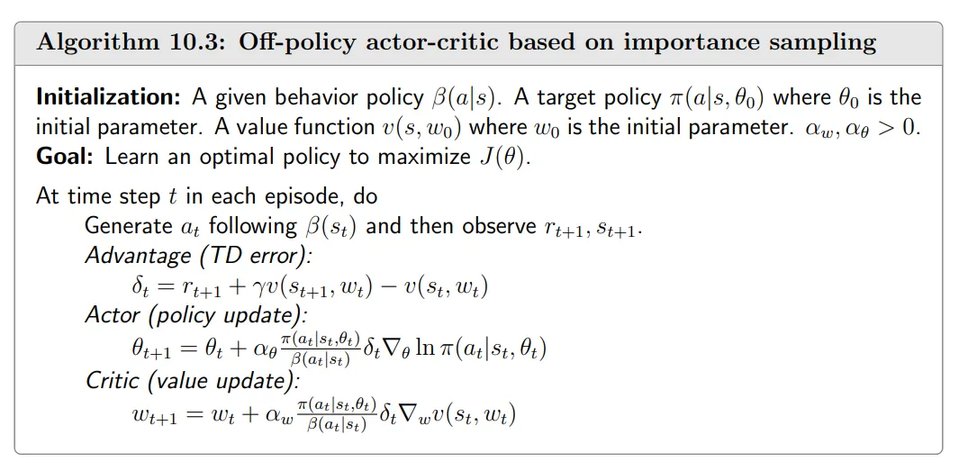
E X ∼ p 0 [ X ] = E X ∼ p 1 [ f ( X ) ] ≈ f ˉ = 1 n ∑ i = 1 n f ( x i ) = 1 n ∑ i = 1 n p 0 ( x i ) p 1 ( x i ) ⏟ importance weight x i . \mathbb{E}_{X\sim p_0}[X]=\mathbb{E}_{X\sim p_1}[f(X)]\approx\bar{f}=\frac{1}{n}\sum_{i=1}^{n}f(x_{i})=\frac{1}{n}\sum_{i=1}^{n}\underbrace{\frac{p_0(x_i)}{p_1(x_i)}}_{\text{importance}\atop\text{weight}}x_{i}. E X ∼ p 0 [ X ] = E X ∼ p 1 [ f ( X )] ≈ f ˉ = n 1 i = 1 ∑ n f ( x i ) = n 1 i = 1 ∑ n weight importance p 1 ( x i ) p 0 ( x i ) x i . The off-policy policy gradient theorem# Suppose that β \beta β β \beta β π \pi π
J ( θ ) = ∑ s ∈ S d β ( s ) v π ( s ) = E S ∼ d β [ v π ( S ) ] , J(\theta)=\sum_{s\in\mathcal{S}}d_\beta(s)v_\pi(s)=\mathbb{E}_{S\sim d_\beta}[v_\pi(S)], J ( θ ) = s ∈ S ∑ d β ( s ) v π ( s ) = E S ∼ d β [ v π ( S )] , where d β d_{\beta} d β β \beta β v π v_\pi v π π . \pi. π .
Theorem 10.1 (Off-policy policy gradient theorem). In the discounted case where γ ∈ ( 0 , 1 ) \gamma \in ( 0, 1) γ ∈ ( 0 , 1 ) J ( θ ) J(\theta) J ( θ )
∇ θ J ( θ ) = E S ∼ ρ , A ∼ β [ π ( A ∣ S , θ ) β ( A ∣ S ) ⏟ i m p o r t a n c e ∇ θ ln π ( A ∣ S , θ ) q π ( S , A ) ] , \nabla_{\theta}J(\theta)=\mathbb{E}_{S\sim\rho,A\sim\beta}\bigg[\underbrace{\frac{\pi(A|S,\theta)}{\beta(A|S)}}_{importance}\nabla_{\theta}\ln\pi(A|S,\theta)q_{\pi}(S,A)\bigg], ∇ θ J ( θ ) = E S ∼ ρ , A ∼ β [ im p or t an ce β ( A ∣ S ) π ( A ∣ S , θ ) ∇ θ ln π ( A ∣ S , θ ) q π ( S , A ) ] , where the state distribution is
ρ ( s ) ≐ ∑ s ′ ∈ S d β ( s ′ ) P r π ( s ∣ s ′ ) , s ∈ S , \rho(s)\doteq\sum_{s'\in\mathcal{S}}d_\beta(s')\mathrm{Pr}_\pi(s|s'),\quad s\in\mathcal{S}, ρ ( s ) ≐ s ′ ∈ S ∑ d β ( s ′ ) Pr π ( s ∣ s ′ ) , s ∈ S , where P r π ( s ∣ s ′ ) = ∑ k = 0 ∞ γ k [ P π k ] s ′ s = [ ( I − γ P π ) − 1 ] s ′ s \mathrm{~Pr}_{\pi }( s| s^{\prime }) = \sum _{k= 0}^{\infty }\gamma ^{k}[ P_{\pi }^{k}] _{s^{\prime }s}= \left [ ( I- \gamma P_{\pi }) ^{- 1}\right ] _{s^{\prime }s} Pr π ( s ∣ s ′ ) = ∑ k = 0 ∞ γ k [ P π k ] s ′ s = [ ( I − γ P π ) − 1 ] s ′ s s ′ s' s ′ s s s π \pi π
Algorithm description# The gradient is
∇ θ J ( θ ) = E [ π ( A ∣ S , θ ) β ( A ∣ S ) ∇ θ ln π ( A ∣ S , θ ) ( q π ( S , A ) − v π ( S ) ) ] . \nabla_\theta J(\theta)=\mathbb{E}\left[\frac{\pi(A|S,\theta)}{\beta(A|S)}\nabla_\theta\ln\pi(A|S,\theta)\big(q_\pi(S,A)-v_\pi(S)\big)\right]. ∇ θ J ( θ ) = E [ β ( A ∣ S ) π ( A ∣ S , θ ) ∇ θ ln π ( A ∣ S , θ ) ( q π ( S , A ) − v π ( S ) ) ] . The corresponding stochastic gradient-ascent algorithm is
θ t + 1 = θ t + α θ π ( a t ∣ s t , θ t ) β ( a t ∣ s t ) ∇ θ ln π ( a t ∣ s t , θ t ) ( q t ( s t , a t ) − v t ( s t ) ) , \theta_{t+1}=\theta_t+\alpha_\theta\frac{\pi(a_t|s_t,\theta_t)}{\beta(a_t|s_t)}\nabla_\theta\ln\pi(a_t|s_t,\theta_t)\big(q_t(s_t,a_t)-v_t(s_t)\big), θ t + 1 = θ t + α θ β ( a t ∣ s t ) π ( a t ∣ s t , θ t ) ∇ θ ln π ( a t ∣ s t , θ t ) ( q t ( s t , a t ) − v t ( s t ) ) , where α θ > 0 \alpha_{\theta}>0 α θ > 0
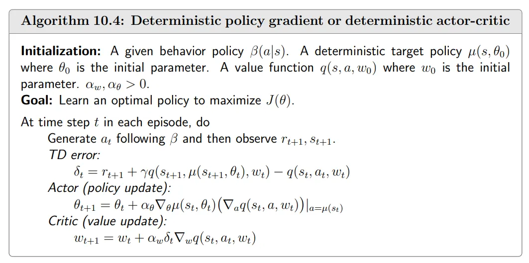
10.4 Deterministic actor-critic# It is important to study the deterministic case since it is naturally off-policy and can effectively handle continuous action spaces .
In this section, we use
a = μ ( s , θ ) a=\mu(s, \theta) a = μ ( s , θ ) to specifically denote a deterministic policy.
The deterministic policy gradient theorem# Algorithm description# We can apply the gradient-ascent algorithm to maximize J ( θ ) J(θ) J ( θ )
θ t + 1 = θ t + α θ E S ∼ η [ ∇ θ μ ( S ) ( ∇ a q μ ( S , a ) ) ∣ a = μ ( S ) ] . \theta_{t+1}=\theta_t+\alpha_\theta\mathbb{E}_{S\sim\eta}\begin{bmatrix}\nabla_\theta\mu(S)\big(\nabla_aq_\mu(S,a)\big)|_{a=\mu(S)}\end{bmatrix}. θ t + 1 = θ t + α θ E S ∼ η [ ∇ θ μ ( S ) ( ∇ a q μ ( S , a ) ) ∣ a = μ ( S ) ] . The corresponding stochastic gradient-ascent algorithm is
θ t + 1 = θ t + α θ ∇ θ μ ( s t ) ( ∇ a q μ ( s t , a ) ) ∣ a = μ ( s t ) . \theta_{t+1}=\theta_t+\alpha_\theta\nabla_\theta\mu(s_t)\big(\nabla_aq_\mu(s_t,a)\big)|_{a=\mu(s_t)}. θ t + 1 = θ t + α θ ∇ θ μ ( s t ) ( ∇ a q μ ( s t , a ) ) ∣ a = μ ( s t ) . It should be noted that this algorithm is off-policy since the behavior policy β β β μ \mu μ